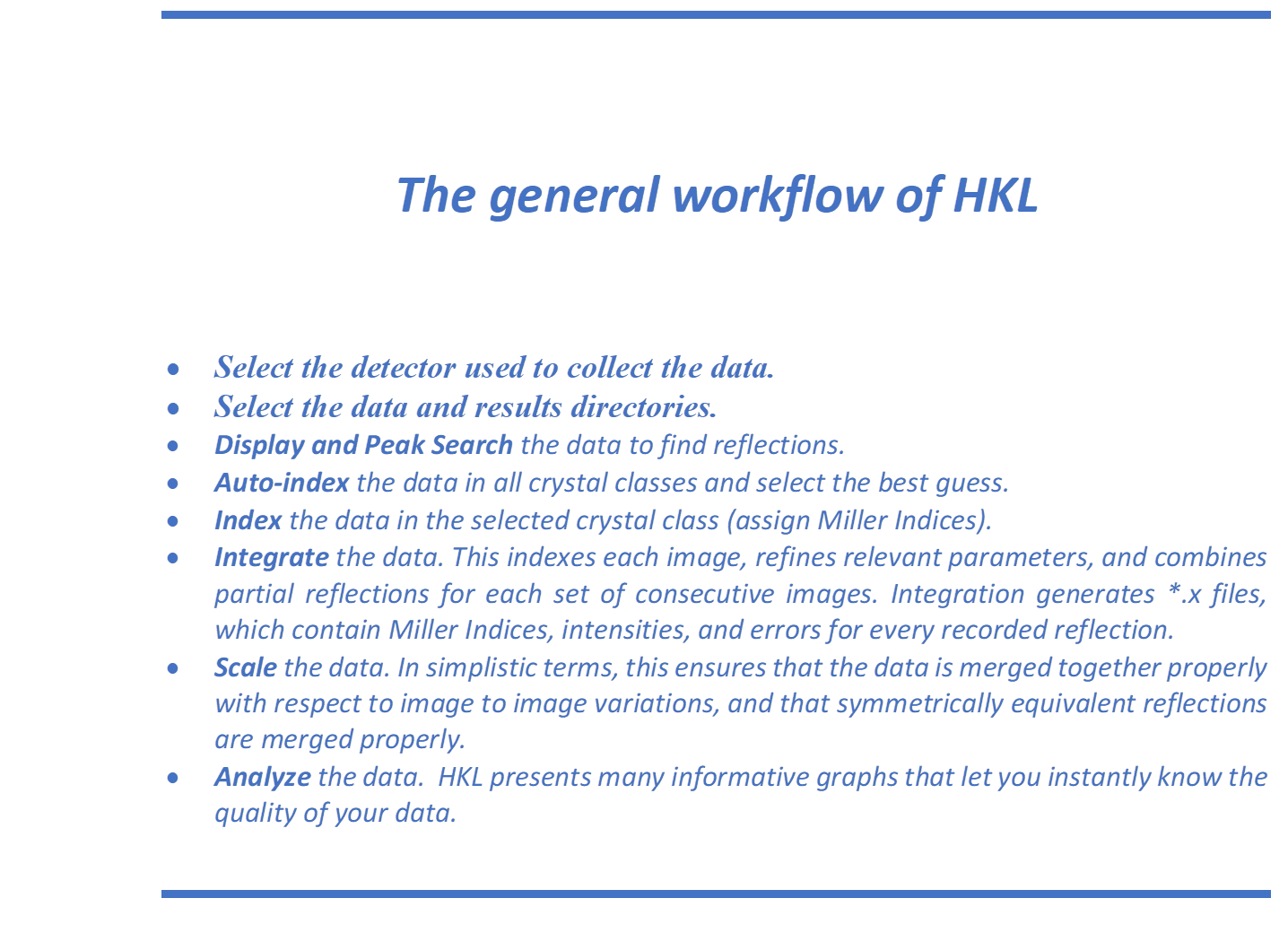
The next few pages show the layout of the different tabs in
HKL-2000, briefly describe the tasks performed on each tab, and provide
information about where in the manual to look for more detailed information.
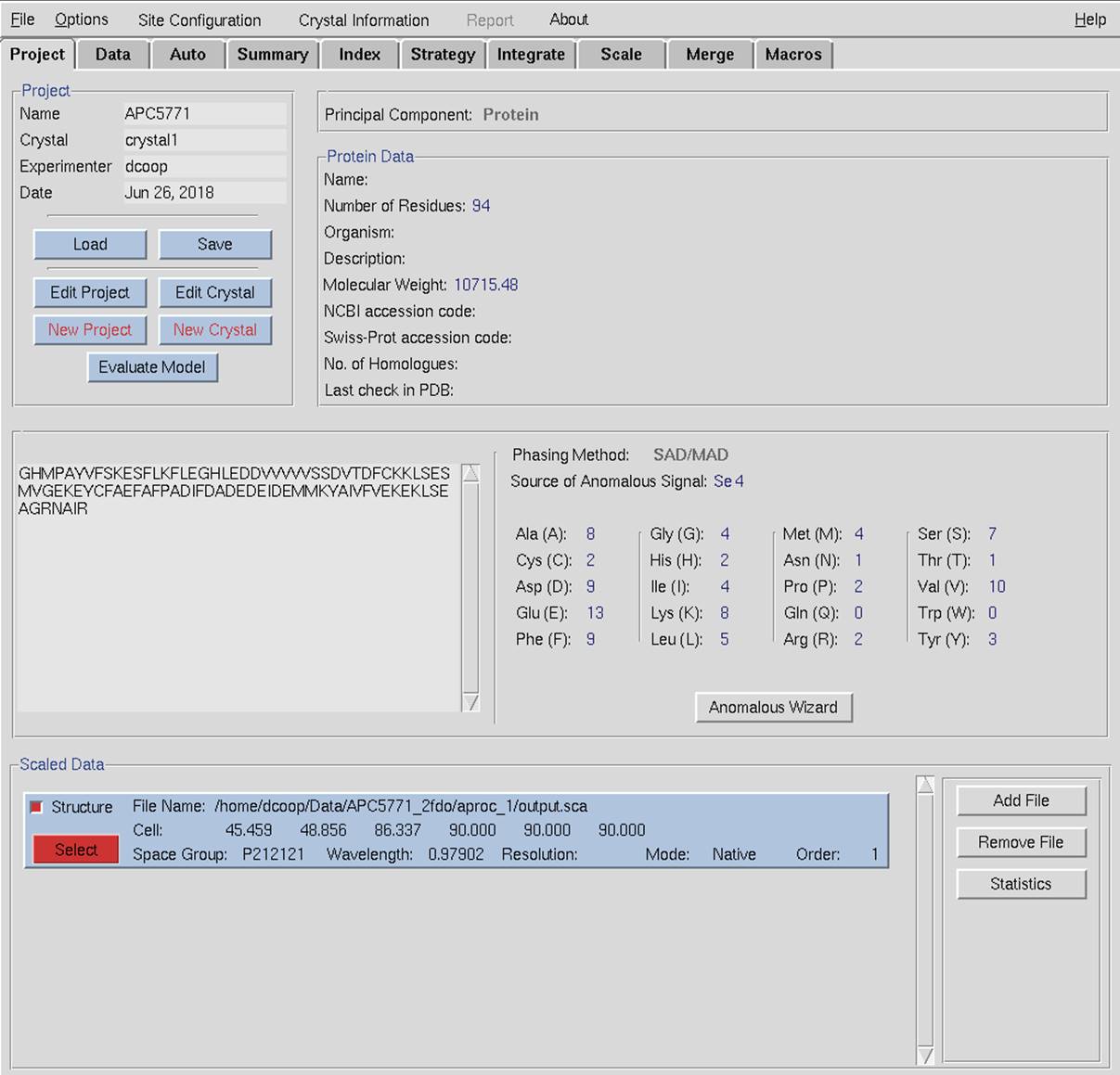
Figure 1. The Project tab contains information about the macromolecule. Using
this tab, you can load or save session information, including which data sets
to work with. Some of the features in the Project tab
are more useful in database linked versions of HKL-2000 and in all versions of
HKL-3000, which requires a database module license. See Create, Save, and Load Projects on page 36 and The Project Tab After Scaling on page 119.
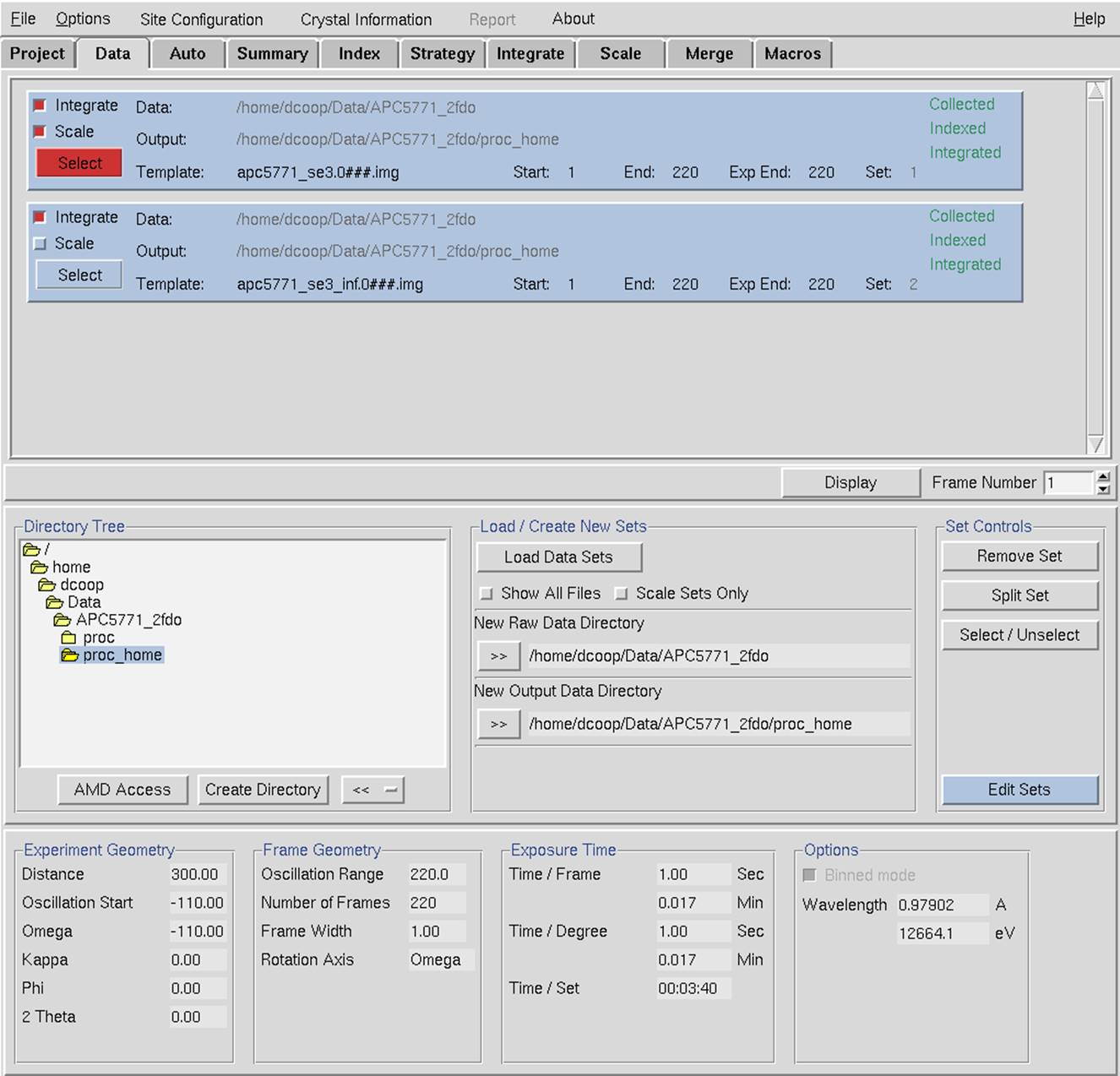
Figure 2. The Data tab displays information about input and output files, displays
information about individual datasets, and has control buttons to work with the
datasets. The top of this tab shows the datasets that you are working with and
what you intend to do with them. The middle of the page allows you to load and
edit the sets you want to use, and the lower part of the display gives
information about the currently selected set. See Data, Results, and Datasets starting on page 25.
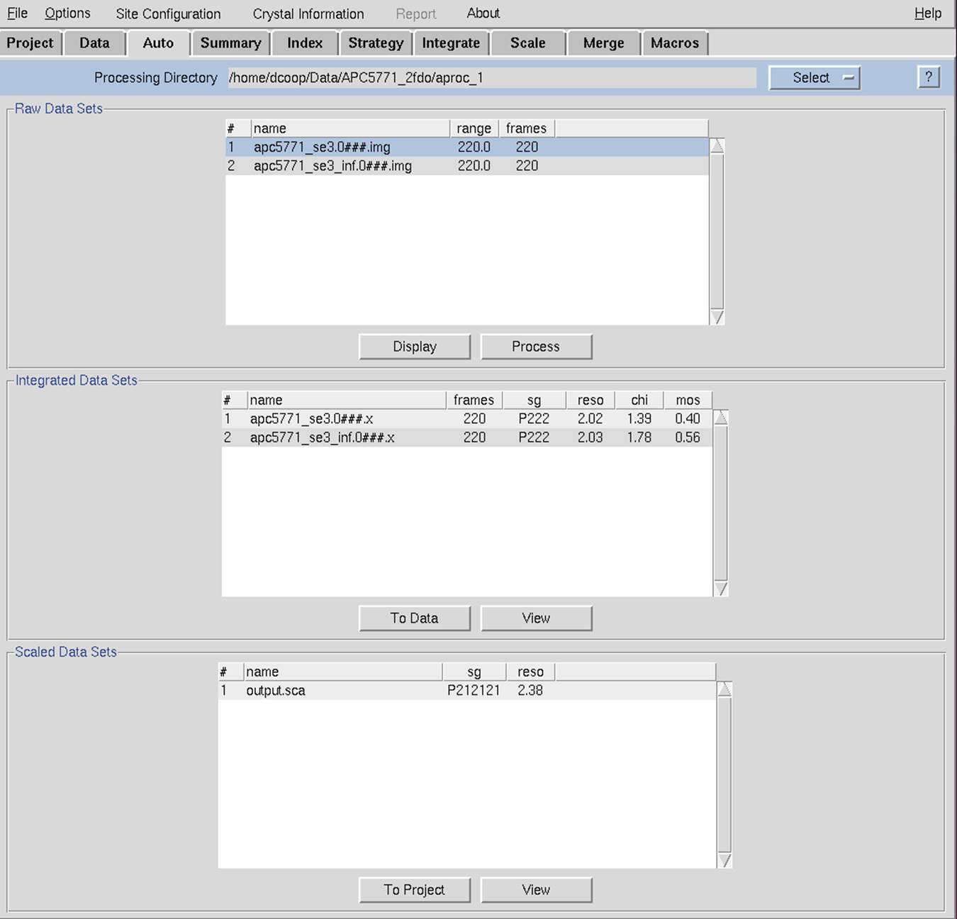
Figure 3. The Auto tab provides you with one-click
processing and scaling your data. See Automatic Data Processing starting on page 121.
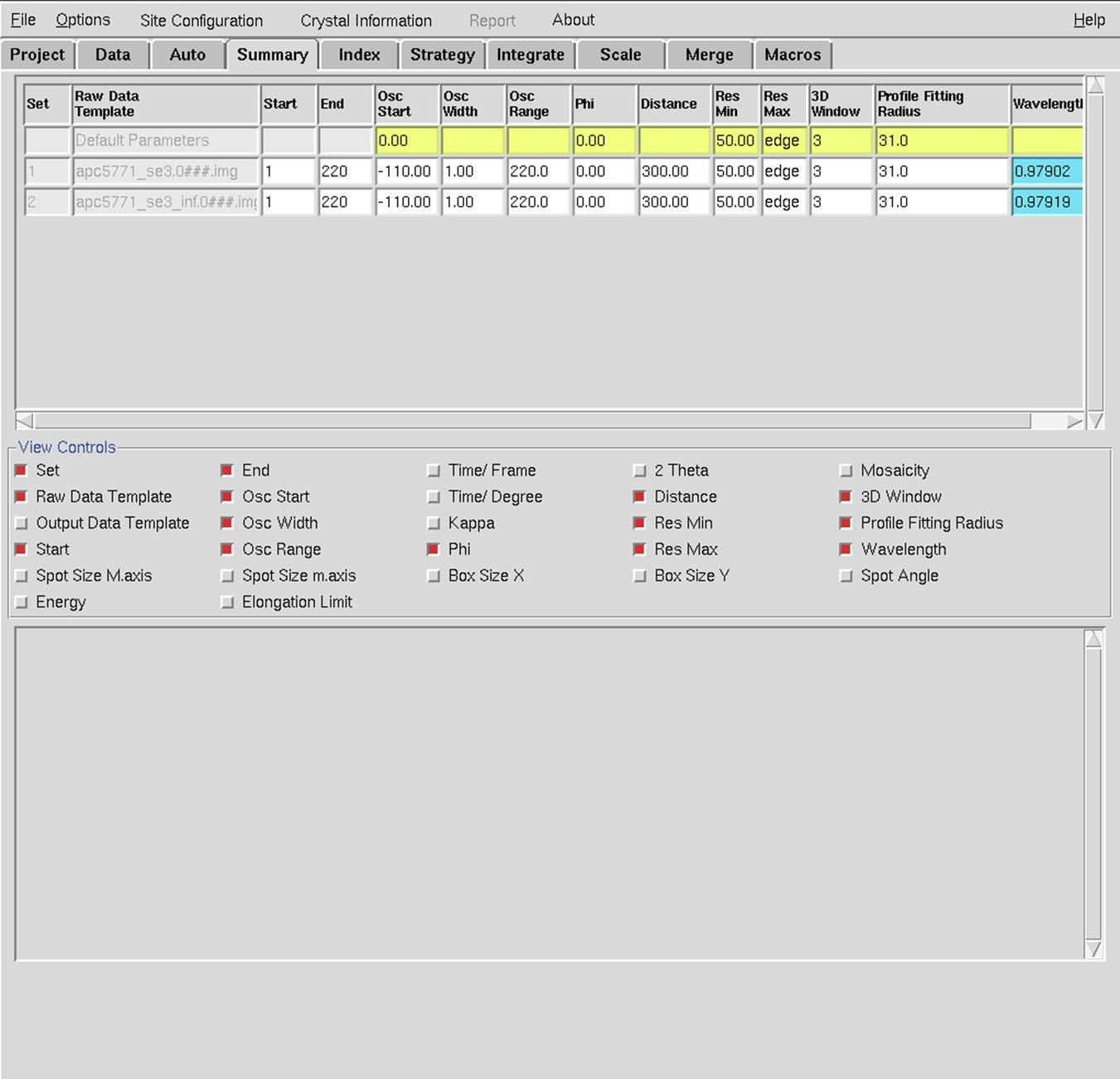
Figure 4. The Summary tab provides detailed information about your datasets and refinement
parameters. Parameters that vary from set to set are highlighted in cyan. The
selector buttons can be used to change which information is displayed in the
table. In this case, these two sets have been collected using the same
strategy, but at different wavelengths. See Checking and Editing Sets on page 32.
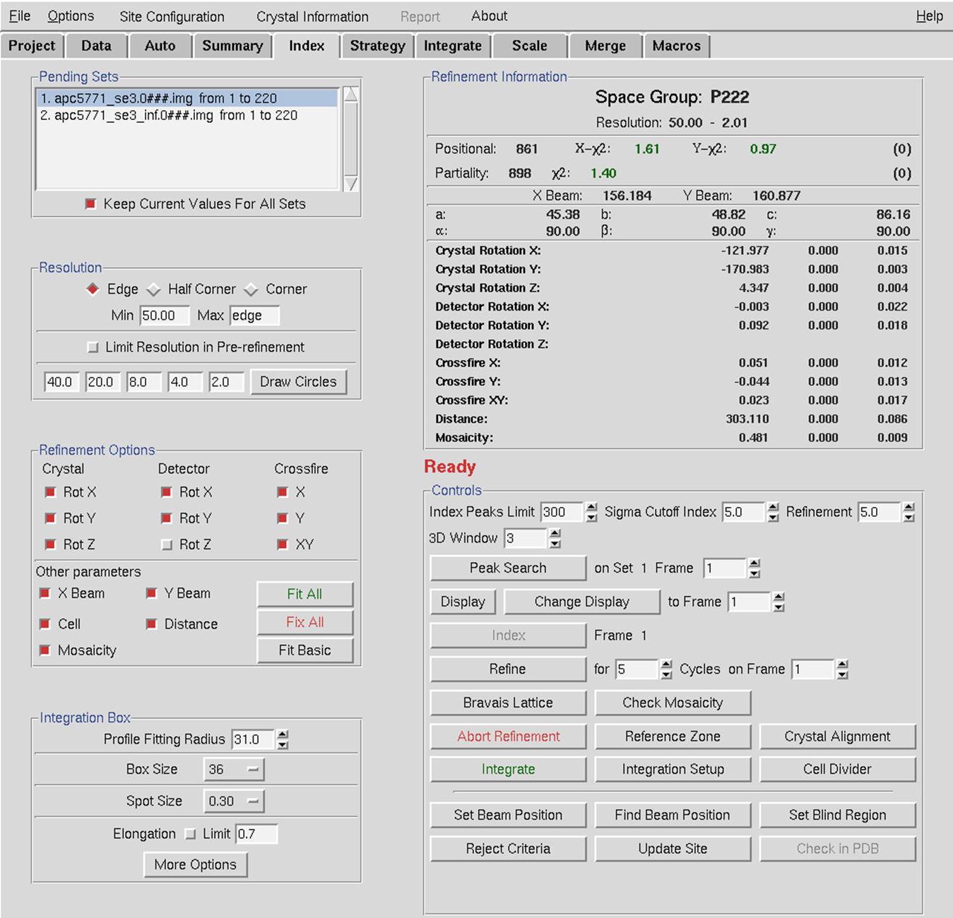
Figure 5. The Index tab allows
you to index your data and refine various parameters. This tab also includes
buttons to mask the beamstop and specify the beam center. In this figure, the
refinement has been completed, and this data is ready to be integrated. The
left side of the display contains control buttons and parameters. The top right
shows indexing statistics and crystal characteristics. The bottom right
contains action control buttons and a few more parameters. See Auto-Indexing starting
on page 52.
The
Strategy Tab
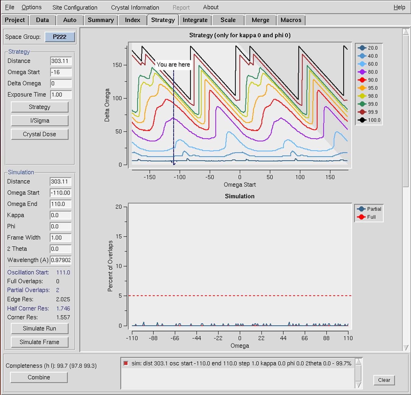
Figure 6. The Strategy tab can help you design your data collection experiment.
An optimal initial orientation will give you a complete dataset before
collecting redundant data, thereby minimizing complications due to crystal
decay. Simulating a run will let you know if you should expect overlapping
reflection, which can severely degrade the quality of your data. See Strategy and Simulation on page 77.
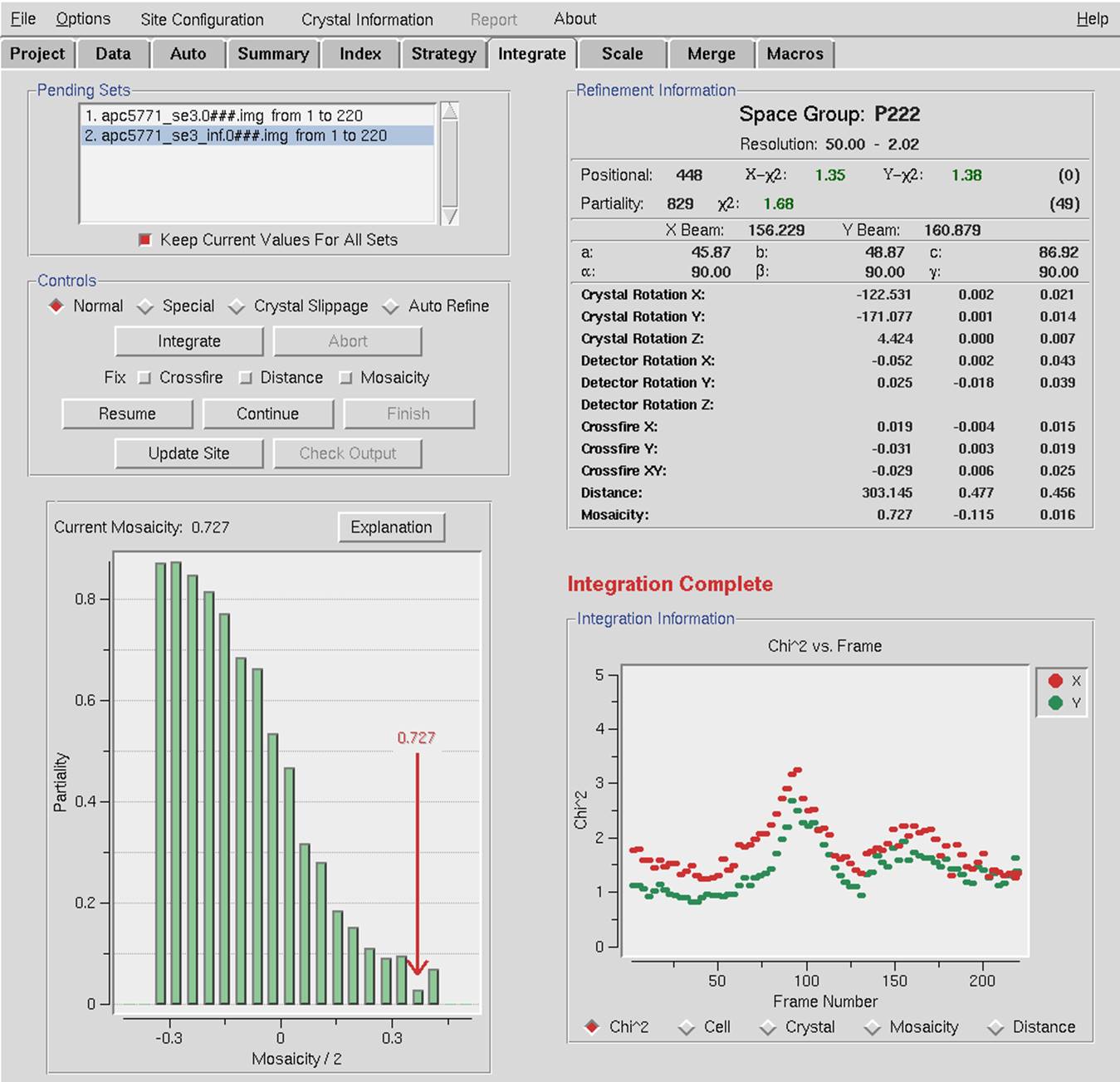
Figure 7. The Integrate tab updates while processing the individual frames.
Refinement information and mosaicity distribution for each frame are shown
along with a graph of how refinement parameters change over the course of the
dataset. See Integrating on page 84.
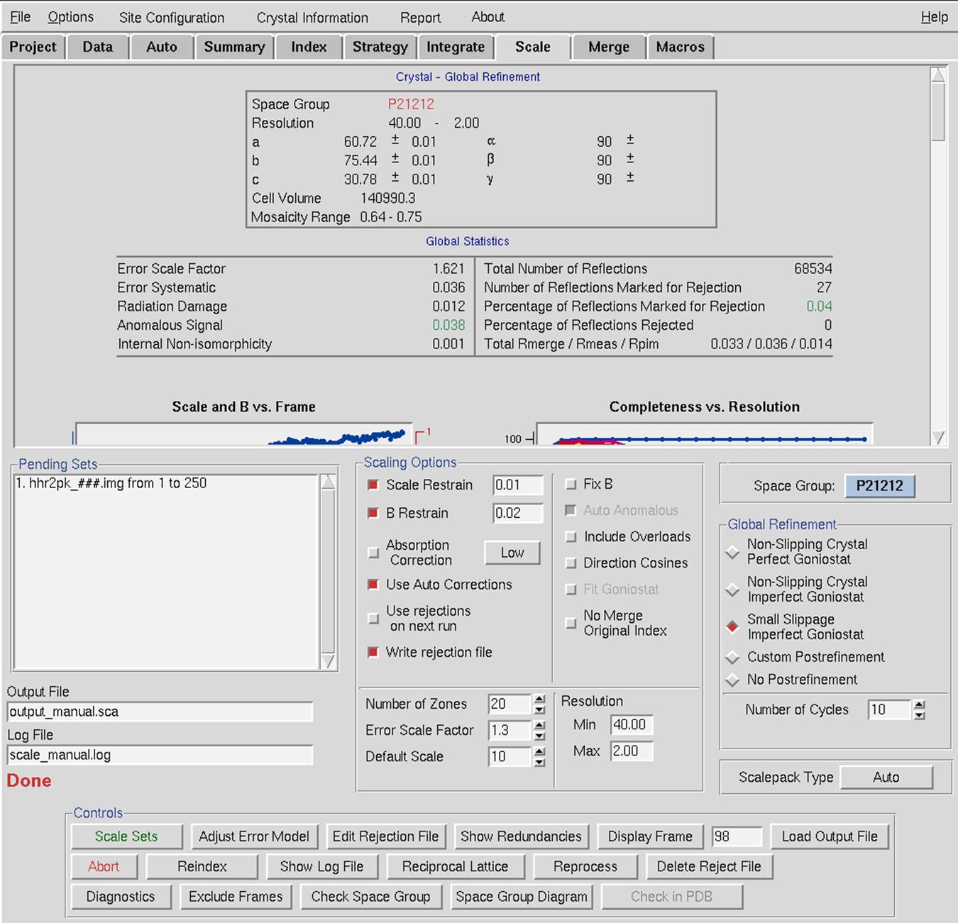
Figure 8. The Scale tab is where you combine all the information from the individual
frames into one Scalepack file (called output_manual.sca in this case), which
contains a unique list of all reflections. Symmetry related reflections have
been merged. The top panel is a scrollable selection of graphs that provide
information about the data quality. The bottom pane lets you control various
parameters or let you inspect results that are not initially displayed. See Scaling on page 90.
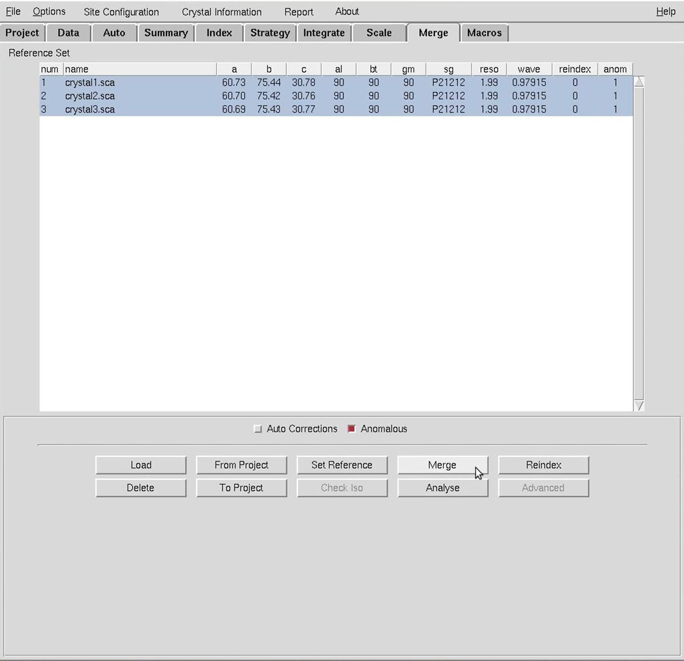
Figure 9. The Merge tab can be used to scale and merge
multiple individually scaled data sets. This allows you to merge data from
different crystals or data that could not otherwise be scaled together. See Merging Multiple Scaled Files on page 124.
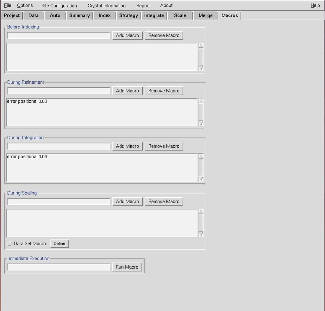
Figure 10. The Macros tab allows you to give specific commands to HKL during various
parts of data processing. The "error positional" macro is one of the more
commonly used macros. It can significantly lower your positional chi2
by allowing more "wiggle room" for your reflections. This is often a detector
dependent necessity. See Using Macros on page 126.
The most critical steps
and information that should not be overlooked are bold, blue, and underlined.
HKL-2000 buttons are in a blue, small caps font.
File names and paths are in a
fixed-width font similar to a Linux console.
Tabs and Options are bold and italic.