
The latest version of the HKL-3000 Tutorial, available below, was prepared by David Cooper and corresponds to the HKL-3000 releases 717 and higher.
This tutorial assumes you have already scaled your data and walks you through the manual process of determining a structure using single-wavelength anomalous diffraction (SAD) data. You can download a printable version of the text found beneath the video with images or the read-along version of the script that has thumbnails aligned with the script for the video. If you still need to process and scale your diffraction data, please see the Indexing and Scaling Tutorial.
Welcome to HKL Research’s “Introduction To Structure Solution Using HKL-3000”. This video focuses on structure solution using single-wavelength anomalous, or SAD, diffraction data. The raw data for today’s tutorial is available at proteindiffraction.org at https://proteindiffraction.org/project/Hhr_1wq6/ . You can search using the keyword ‘Workshop’ to find several excellent data sets. The one that we will work with today is 1WQ6, the nerve homology 2 domain of ETO. When you download the data from proteindiffraction.org, it will come with the site file that defines the detector setup.
This tutorial assumes that you have already scaled your data. See the links below for detailed tutorials for scaling the data in either an automatic or manual procedure. For today’s tutorial, I will load already processed data using the Load button in the Project tab. Notice that loading this project will load a scaled set into the Scaled Data window.
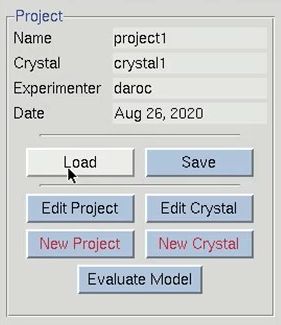
The structure solution module of HKL-3000 needs to know some basic information about your project in order to help you solve the structure. I could have saved this information before and loaded it when I loaded the data, but left it out to show the data entry process. Click the Edit Project button to load the necessary information.
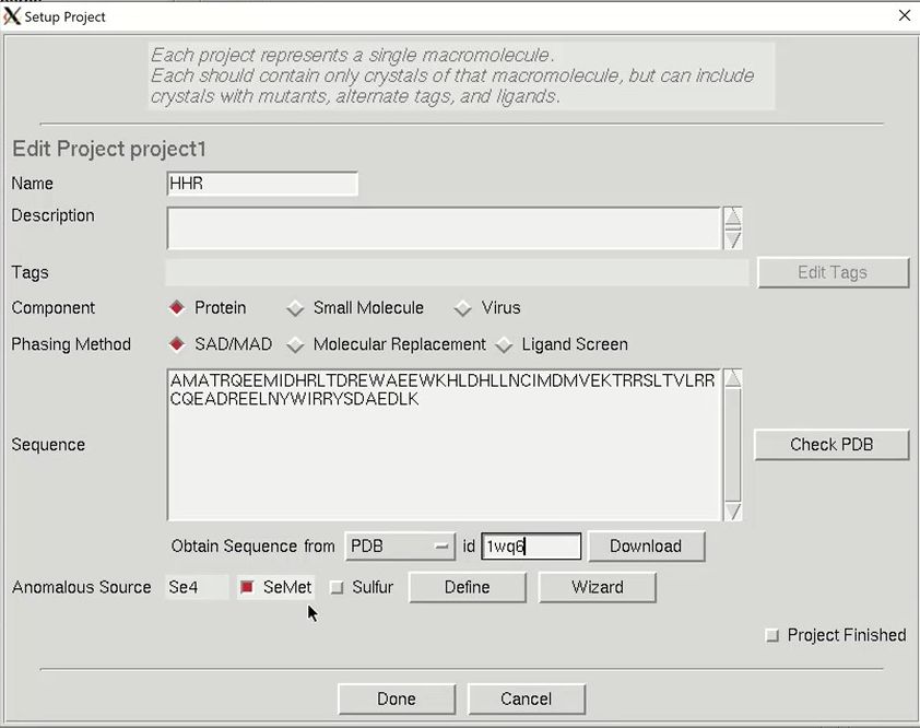
The minimal information that HKL needs is the type of macromolecule you are working with, the phasing method, the sequence, and the source of the anomalous signal. Although you can cut and paste the sequence, HKL can import it and some other information from several databases. Select the database using the drop-down menu labeled Obtain Sequence From and type the id associated with that database in the id field. Click download to fetch the sequence. The amount of data filled out in the tab is dependent on which database you use to obtain your sequence.
We will solve the structure using selenomethionine, so select the SeMet option, which will fill in the anomalous source field and the number of seleniums. However, if we were working with another heavy atom, we could have selected Define to select an element from the periodic table. The wizard can be used to see anomalous scattering curves. Close the “Setup Project” dialog by clicking Done. The completed information now appears in the Project window.
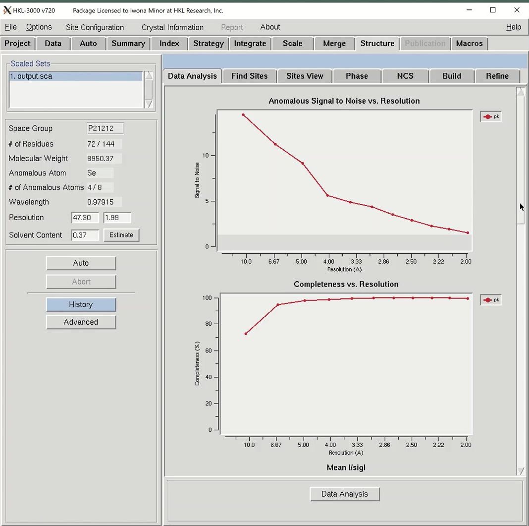
We are now ready to solve the structure using the Structure tab. Because we have defined the phasing method as SAD/MAD, the contents of the Structure tab will be specific for this method. On the right, we see some information about the project. Most of this is either set or based on information in the Project tab.
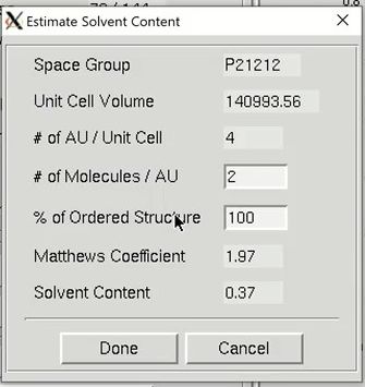
HKL-3000 will automatically estimate the number of molecules in the asymmetric unit (ASU), the Matthews coefficient and the solvent content. You may override the number of molecules in the asymmetric unit by clicking the Estimate button, which opens a new window. Changing the number of molecules will recalculate of the solvent content and the Matthews coefficient. The calculated values will appear in red if they are unusual and possibly incorrect. Changing the percentage of the molecule with ordered structure does not change the solvent content and the Matthews coefficient, but does change the number of residues sent to the model building procedures. Changing the number of molecules in the ASU will also change the number of sites that will be searched for. If the anomalous source is selenomethionine (SeMet), an N-terminal SeMet will be omitted from the automatic count, as it is presumed that the initial SeMet residue is cleaved or disordered. You can also change the resolution you want to use for structure solution, although the defaults are usually sufficient.
Underneath this information is the Auto button, which will run the automatic structure solution and model building procedure. This procedure will work in most cases, but this tutorial will manually go through the process to ensure you are familiar with what the Auto process will do.
To the right are tabs for the different stages of structure determination. The first step to solving the structure is to analyze the data, so click the Data Analysis button at the bottom of the window. Data analysis of the diffraction data is provided by the SHELXC and TRUNCATE programs. The results are shown in several graphs.
The “Anomalous Signal to Noise vs. Resolution” plot shows the presence or absence of anomalous signal in different resolution shells as measured by the signal-to-noise ratio (SNR) calculated by SHELXC. The gray shaded region on the graph shows SNR values below 1.3, where the anomalous signal is probably insignificant. The data used here has an extremely strong anomalous signal.
After analyzing the data, we are ready to move on to solving the heavy atom substructure using the Find Sites tab. HKL uses SHELXD for the substructure solution. To start the process, first adjust the resolution to reflect the strength of the anomalous signal from the Analysis tab. Then click Find Sites to start the substructure solution. Including high-resolution data without a significant anomalous signal will only add noise to the substructure search process. The graphs presented on this tab come from the SHELXD output.
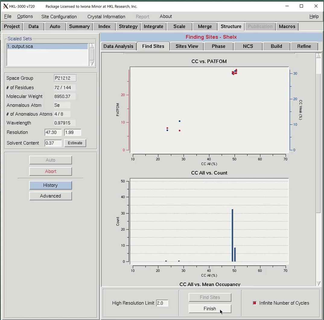
The most important graph is the “CC vs PATFOM,” which plots both the Correlation Coefficient (CC) of weak reflections (blue dots) and the Patterson figure of merit (red dots) as a function of the CC of all reflections. Two things are important when searching for good substructure solutions. First, all three values (CC All, CC Weak, and PATFOM) for the best solutions should be significantly greater than the corresponding values for other solutions. Second, there should be clear separation between the best solutions and the large population of non-solutions, which may be more clearly seen when Infinite Number of Cycles is selected.
The program will search for substructure solutions until it finds one with CC All above 30 and a CC Weak above 15. These will appear as points in the upper right of the graph. This data is very strong, so this process may not take long. When using weaker data, check the Infinite Number of Cycles box to instruct SHELXD to keep searching for sites. When using this option, you will be required to press the Finish button when you are satisfied you have found an adequate substructure.
The second plot “CC All vs. Count” shows a histogram of the CC All percentages for all solutions calculated, which may be used to determine the relative size of each cluster of solutions. From that plot, you know how many times a particular solution occurs.
The third plot “CC All vs. Mean Occupancy” shows the mean occupancy for all sites in for each substructure solution as a function of CC All. SHELXD uses relative occupancies, where the strongest site (or atom) in the substructure is assigned occupancy 1.0, and the other sites are scaled relative to the first.
The results of substructure determination, as calculated by the Find Sites tab, are displayed on the Sites View tab. The sites of the solution are displayed in a three-dimensional representation of the unit cell. Sites will be displayed as blue spheres with their size proportional to their occupancy. The fractional coordinates and relative occupancies of these site will appear in the table at the bottom of the page. The 3-D display of the sites may be rotated by left-clicking and dragging on the window, and zoomed in or out by right-clicking and dragging. This display can be helpful for detecting split sites and possible non-crystallographic relationships. Buttons are available to display symmetry related sites and sites related by non-crystallographic symmetry. This latter button will only work after using the NCS tab.
The solution that is initially selected will be the “Best” structure solution, as judged by the CC All, CC Weak and PATFOM values. Other potential solutions are listed in the box at the top of the page. The solution sets can be sorted either chronologically (select the Last button) or by the strength of the solution (select the Best button). When you select another set with the mouse, the sites from that solution will be displayed as red cones, with the size of the cone proportional to the relative occupancy of that site. Viewing the sites does not automatically change the sites that HKL will work with. In order to actually change the sites for the overall structure solution, you must click the Use Sites button. This button converts the red cones into blue spheres and populates the table of sites at the bottom of the page with the sites of the selected solution.
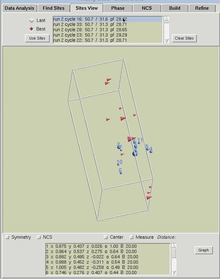
The table at the bottom of the page can be used as an interactive means of selecting which sites should be used for phasing. Click the Graph button to display the table in a graphical format. Moving the mouse over the graph will display crosshair lines. When you click the mouse, the relative occupancy associated with the mouse position will be printed under the Delete button. Clicking the Delete button will remove sites with an occupancy lower than the selected value.

Some less commonly used features relating to substructure solution, such as setting the minimum site-to-site distance, identifying the number of disulfides bridges, allowing sites in special positions, etc. may also be accessed through the Advanced button in the left sidebar. The “Advanced Mode” dialog also permits saving or loading substructure atom positions to a file.
Once you have determined which set of sites you would like to work with, switch to the Phase tab. The information on the left side of the page will stay the same. The top of the right side will initially be empty, but will display the phasing statistics once you start the phasing process. The control buttons are in the bottom panel. You can change the high-resolution limit for phasing using the resolution field on the left. You should note however, that although this limits the reflections used in phasing (run by MLPHARE), the phases will be extended to the full resolution of the data via phase extension. If you truly want to limit the resolution of the solution, you should rescale your data to that resolution.
Before the data is phased, you first have to determine if the sites have the correct hand because the sites determined in the previous tab have an equal chance of being correct or having an inverted hand. Therefore, before the data is phased, it is important to check the hand of the solutions. Use the Check Hand button to do this. HKL-3000 will run SHELXE twice to calculate and refine two sets of electron density maps, using phases from either the original substructure or the same substructure with positions inverted (i.e., the opposite hand).
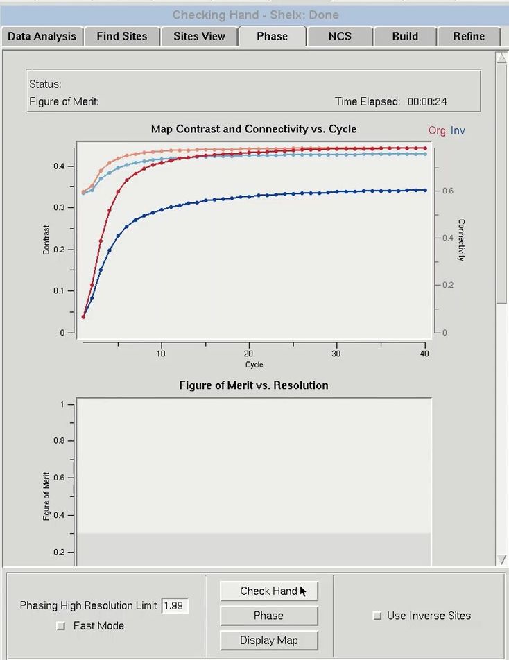
The results from phasing using both hands will appear in the top graph (“Map Contrast and Connectivity vs. Cycle”). Statistics for the map calculated from the original sites are red, and the map from the inverted sites are blue. Two different parameters are shown. The darker lines (red and blue) are the map contrast and the lighter lines (pink and light blue) are the map connectivity. If you have a valid solution, the map contrast of one of the two substructure hands will be much higher than the opposite hand, and this is presumed to be the correct hand. In cases where the inverted hand is the better solution the Use Inverted Hand option will automatically be selected.
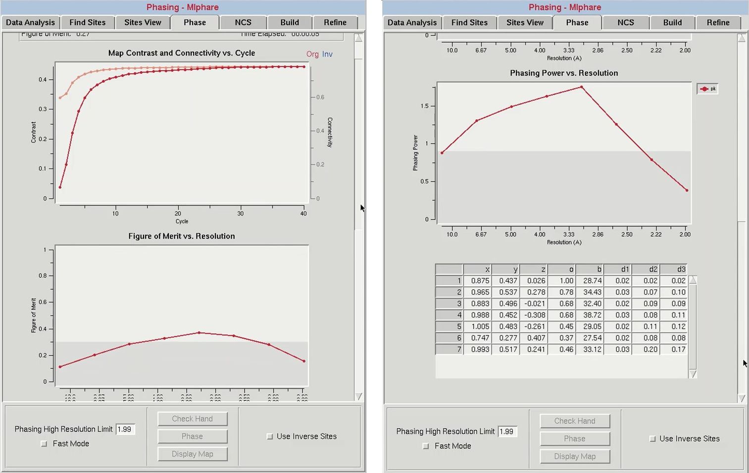
After determining the proper handedness for the substructure, click the Phase button to calculate the experimental phases. This will run the programs SHELXE and MLPHARE sequentially. First, the SHELXE run will be repeated using the selected hand, and the substructure will be improved in MLPHARE. This will refine the coordinates, occupancies, and B-factors for the substructure atoms and use the refined positions to generate phase information. Statistics from phasing will be displayed in two plots: “Figure of Merit vs. Resolution” and “Phasing Power vs. Resolution.” The table at the bottom will display the current values of the substructure coordinates, occupancies, and B-factors. When phasing is complete, maps and the substructure sites will be displayed in Coot. You may have to use the “Go To Atom” option to find the substructure. The experimental density map will be displayed in blue and the anomalous density map will be displayed in orange. The peaks of the anomalous density map should correlate with the sites.
Within the “Figure of Merit vs Resolution” plot, the red line shows the mean figures of merit (FOM) values for the MLPHARE-calculated phases by resolution shell. The blue line shows how the mean FOM is improved by density modification, and this line should appear higher than the red line. This plot is dynamically redrawn through subsequent runs and cycles of refinement.
The “Phasing Power vs. Resolution” displays the mean “phasing power” by resolution shell. Phasing power values greater than 0.9 are considered to be significant, and accordingly the region of the plot below 0.9 is marked in gray. If the line dips into the gray area at higher resolutions, consider limiting the high-resolution limit of phasing. All of the data will still be phased through phase extension.
If you have more than one copy of the molecule in the asymmetric unit, you may use non-crystallographic symmetry (NCS) for a phase improvement. However, this particular set of data does not have non-crystallographic symmetry and this function is not covered in this tutorial.
Once phasing is done and you have produced a reasonable electron density map, click the Build tab to start model building. HKL-3000 includes several options for the program it will use to build the structure. Buccaneer is currently the default program. ARP/wARP and Resolve are available if you have them installed, and Nautilus can be used for nucleic acids. I suggest using HKL Builder, which uses Buccaneer and carefully selected default options that have given us the best results in many cases. Some program options may not be available if they are not installed on your computer. An Auto button is available to complete the process with limited interaction, but the main process is so efficient, it is not really necessary.
Before starting the building cycle, you may change the number of model building cycles in the main window. The One Cycle checkbox can be used to build a preliminary model quickly to verify if the structure solution is correct. The Use Sequence option will determine whether or not the building program has access to the sequence that is stored in the project tab. If you deselect this option, you will only be able to generate a C-alpha trace.
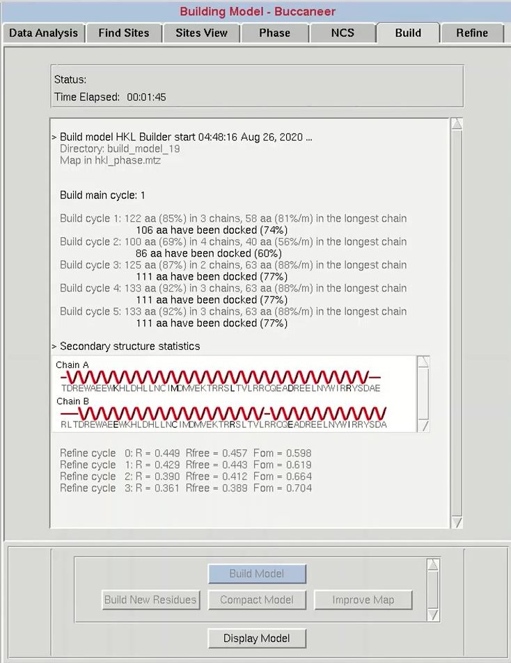
The progress of the building process will be displayed in the main window as the building progresses. For each cycle, the number of residues built and docked will be displayed, as well as the number of chains that contain them. After each main cycle, the secondary structure of the current model will be displayed along with the sequence. This does not mean the sequence has been used in the building process, which is controlled by the Use Sequence button. Each cycle of building will be followed by rounds of refinement in Refmac, and the R-values and the FOM from these cycles will be displayed. If things start to go wrong during the building process, you can use the Abort button to stop the process and save time.
After model building is complete, HKL-3000 starts Coot to display the current model, the substructure atoms, the 2Fo-Fc map, the Fo-Fc difference map, and the experimental phase electron density maps. In basic cases where the initial electron density map is of high quality, you may build an almost complete model. However, when you have low resolution data or there is some problem with phasing, the initial model will be incomplete.
As with other tabs within the Structure tab, you may modify the default parameters of the computations in the “Advanced Mode” dialog (below). For example, you may define the number of REFMAC refinement cycles between building cycles.
All of the tabs within the Structure tab have a History button, but its utility first becomes apparent when you are building models. All files (*.pdb, *.mtz, etc.) created by the model building process are stored in a numbered build_model directory. By default, the list of files that appear in the “HKL file” and “PDB file” pulldowns are in the most recently created directory. However, if you close and restart the program, or if you go back and calculate new experimental phases on the Phase tab, the next time you click Build Model on the Build tab, a new build_model directory will be created and the old models and structure factors from prior sessions will no longer be accessible in the file pulldowns. The “History” button allows you to return to a previous session. For example, if the current session is build_model_17, but better models were built in the prior session build_model_12, clicking “History” and selecting the earlier session changes the contents of the pulldowns to list the files from the prior session directory.
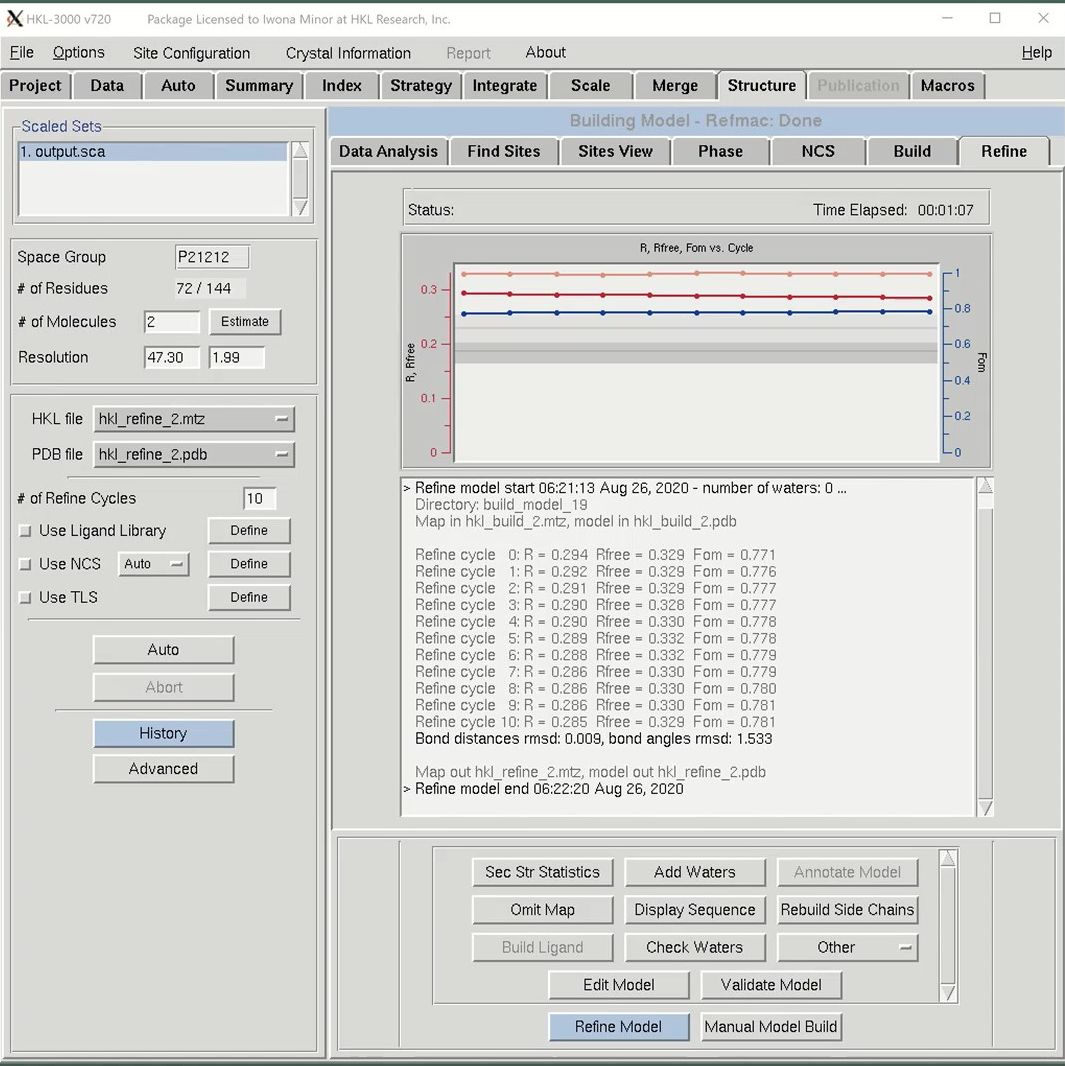
After building an initial model, you may use the Refine tab to do subsequent iterative refinement of your structure. REFMAC will be used to perform refinement using the files selected in the “HKL file” and “PDB file” dropdowns. The Refine Model button will perform the number of cycles indicated in the “# of Refine Cycles” selector. The “R, Fom vs. Cycle” plot in the top of the window will render a plot of Rfree factor (orange), R factor (red) and mean figure of merit (blue) by cycle. This is a cumulative graph, so subsequent rounds of refinement will be added to the previous rounds. This lets you see the progress of the project, not just this particular round of refinement. Results of the individual cycles of refinement are shown in the window under this graph, as are the overall statistics and file names for each round of refinement. When a round of refinement is done, the resulting files will automatically populate the “HKL file” and “PDB file” dropdowns.
Use the Manual Model Build button to open the model and maps in Coot. If you make any modifications, save the file to the current working directory and it will become one of the options in the PDB file dropdown list. Be sure to select it before performing the next round of refinement.
If ligands or non-standard residues are present in the model that require custom restraint libraries, check “Use Ligand Library” and click “Define” to either explicitly choose a ligand restraint library (in *.cif format), or to generate new restraints from a ligand structure using LIBCHECK. If you get these files from another source, copy them into this session directory and select it using the Define button.
The Use NCS option controls whether NCS restraints are used during refinement. In “Auto” mode, the REFMAC will attempt to determine which residues are related by NCS automatically. In “Manual” mode, the ranges of residues related by NCS are manually specified with the “Define” button.
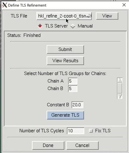
The Use TLS option controls whether anisotropic Translation-Libration-Screw motion refinement of rigid domains or fragments of the model should be performed. To use TLS refinement, the rigid groups must be assigned using the “Define” button. The TLS groups can be supplied manually, but a good approach is to use the TLS Motion Determination (TLSMD) server. The server can be found online, but HKL provides a convenient Submit button. This will open a web browser and go to the results from the TLS Motion Determination server. Back in HKL-3000, select the number of TLS groups you would like to divide each chain into and select Generate TLS. You can optionally reset the B-factors when you generate the TLS groups. Here you can change the number of TLS refinement cycles to be performed. If you want to use previously refined TLS parameters without refining them, which can save time during later stages of refinement when the TLS parameters have stabilized, select the Fix TLS option.
Other parameters that control the operation of REFMAC may be adjusted through the “Advanced Mode” dialog, which are described in more detail in the REFMAC manual and are beyond the scope of this introductory tutorial.