|
HKL-2000 Online Manual |
||
|
Previous Integration |
Table of Contents | |
Scaling
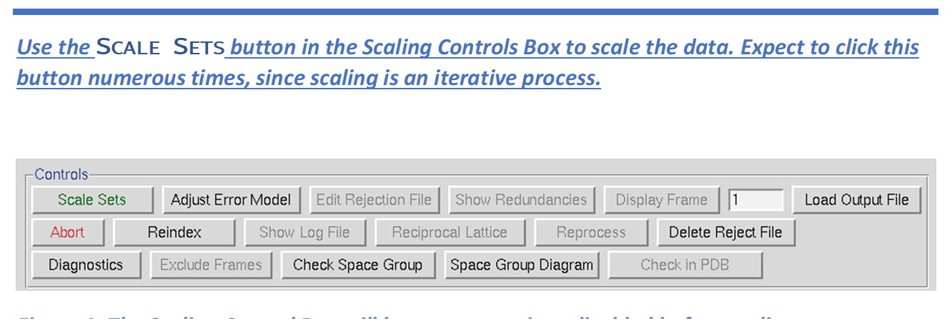
The Scale tab provides the interface to the Scalepack program. This window is divided into three sections. The top of the window is reserved for the results and analysis of the scaling process and will be blank until after the first round of scaling. The middle section contains a control panel with options that can be changed before or (and after) scaling the initial round of scaling. The bottom of the display contains the scale sets button and a set of controls that only make sense after at least one round of scaling (they are actually not available at first). It is important to know that scaling is an iterative process. To get high-quality data, you will have to scale the data multiple times, adjusting some parameters based on the results of the last round of scaling.
Under most circumstances, the default options will be sufficient to start the scaling process, although you should make sure the Anomalous option is checked if you are conducting a SAD or MAD experiment. It will be set by default if you have selected SAD/MAD as the Phasing Method for the project, but will not be selected if you have jumped into data processing without defining the project. The default Global Refinement choice (Small Slippage and Imperfect Goniostat) should be suitable for most cases, but you do have the option of selecting a different option (see the Post Refinement box below for more details).
Scaling Options
These options affect how the scaling of the integrated diffraction intensities is performed. The default options are: Scale Restrain 0.01, B restrain 0.1, Write Rejection File, Ignore Overloads, Number of Zones 10, Error Scale Factor 1.3, Default Scale 10, and Resolution Limits as determined from the *.x file headers (Figure 86). What follows is a discussion of each of the options listed in this panel.
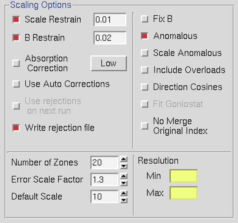
Figure 86. The Scaling Options panel
Scale restrain can be used to restrain scale factor differences from consecutive films or batches. The value entered in the box represents the amount you will allow the scale factors to differ from consecutive frames or batches. It adds a factor of (scale1 - scale2)2/(scale restrain)2 to the target function minimized in scaling. This only applies to batches between which you add partials. The value should roughly represent the expected relative change in scale factors between adjacent frames.
For very thin frames, or frames where most of the reflections are partially recorded (yellow, as opposed to green, spots on the image during integration, see Figure 48), or in sectors whose width is less than the mosaicity, or from data which consists of only a few frames, scale restrain is almost obligatory. In these cases, there may not be enough intersections between frames to get accurate scale and B factors. Indeed, what you may see is both scale and B factors ranging all over the place. If things get really bad, the program may crash due to floating-point arithmetic exceptions when taking the exponent of unreasonable B factors. This does not mean that the data is unusable; it simply means that the scale and B factors must be restrained. Note that the restraints only apply to the frames over which you are adding up partially recorded reflections.
It is not correct to try to "bin" the individual frames into larger batches to try to overcome the problem of few intersections between frames. This is because you then lose the ability to add partials between the new "bins." You can, however, overcome the problem in another way, by adding the macro number of iterations 0 to the During Scaling box on the Macros panel. In this case, the data will not be scaled but simply merged. This has its drawbacks.
B Restrain can be used to restrain B factor differences from consecutive frames or batches. The value which follows the flag represents the amount in Å2 you will allow the B factors to differ from consecutive frames or batches.
Absorption Correction applies additional parameters that correct for variations in the degree of X-ray absorbance by the crystal in different orientations. For example, more X-rays are absorbed when the longer dimensions of the crystal are parallel to the incident beam. In essence, this procedure adjusts for the fact that most crystals are not perfect spheres! The absorption correction algorithm parameterizes this effect by an expansion of real spherical harmonics terms (the Low or High option controls how many terms are included in the correction). This procedure, along with several other scaling corrections applied by Scalepack, is described in more detail in Otwinowski et al. Acta Cryst A59: 228-234 (2003).
In the majority of cases, there is likely to be the improvement of the quality of the scaling results (and no harm!) in including at least Low absorption corrections. The only serious drawback is in the speed of the scaling process, as Scalepack requires additional processing time to calculate the spherical harmonic expansions.
Use Auto Corrections can help determine difficult structures, but the resulting reduced data should not be used for refinement or deposition. This option automatically adjusts the error model, which can be especially useful with weak anomalous signals or anisotropic diffraction. This option reliably models correlated errors and is generally better than manually adjusting the Error Scale Factor and Adjust Error Model options. It is a good practice to add "auto" to the results filename to remind yourself not to refine against this data.
Use Rejections On Next Run means that the reflections that were written to the file reject are not used in subsequent scaling runs. Unless this is explicitly checked, reflections will only be flagged for rejection, not actually rejected. Generally, one uses this on the second and all subsequent runs of scaling. It does not hurt to have this option selected if there is no reject file (i.e., your first run or after deleting the file).
Write Rejection File tells the program to create a list of reflections, stored in the file called reject that meet the criteria for rejection. They are applied, i.e., rejected, when the use rejections on next run button is checked. If you make changes to the error model or make a change the space group that would merge different reflections, you will need to remove the reject file using the delete reject file in the control box at the bottom of the page.
Fix B tells the program not to fit B factors at all. Usually, it is combined with the input of the B factors you want to apply but do not wish to refine anymore, or it is used for frozen crystals where you do not expect significant decay. This is in contrast to the default procedure, where the B factors are fit only after the convergence of the scaling. In the default procedure, if scaling does not converge in 20 (default) cycles of refinement, B factors will not be fitted.
Anomalous. This flag keeps Bijovets (I+ and I-) separate in the output file. If the Anomalous flag is on, anomalous pairs are considered equivalent when calculating scale and B factors and when computing statistics but are merged separately and output as I+ and I- for each reflection. See the next section for a discussion of how to treat data that contains an anomalous signal.
Scale Anomalous. This is the flag for keeping Bijvoets (I+ and I-) separate both in scaling and in the output file. If the Scale Anomalous flag is on, anomalous pairs are considered non-equivalent when calculating scale and B factors and when computing statistics, are merged separately, and output as I+ and I- for each reflection.
This is a dangerous option because scaling may be unstable due to the reduced number of intersections between images. The danger is much greater in low symmetry space groups. Scale Anomalous will always reduce R-merge, even in the absence of an anomalous signal, because of the reduced redundancy. However, &chi2 values will not be affected in the absence of an anomalous signal.
Include Overloads. "Overloads" are reflections that contain pixels that exceed the maximum measurable intensity and will have an intensity is set at the maximum intensity possible for the detector. Since the intensity of these pixels cannot be determined accurately, the default behavior is to ignore reflections that contain overloads. In some cases, you may want to retain the reflections that if only a few pixels exceed the maximum. If this option is selected, fitted profiles with missing pixels (typically due to overload) will be included in the scaling.
Direction Cosines produce information that can be read by an outside absorption correction program, such as Shelx. Generally, this option is not needed as HKL-2000 is capable of applying absorption corrections intrinsically (see above).
Fit Goniostat gives the goniostat misalignment angles. It should only be used by beamline staff or the maintainers of X-ray diffractometers.
No Merge Original Index will disable the default behavior of merging reflections; thus, reflections with the same unique hkl will not be combined. Furthermore, the output will also contain the original (not unique) hkl for each reflection. This option can be useful if you would like to examine the indexed, but unmerged data, in an external program. This may be useful when determining the space group is difficult. The output will consist of the original hkl, unique hkl, batch number, a flag (0 = centric, 1 = I+, 2 = I-), another flag (0 = hkl reflecting above the spindle, 1 = hkl reflecting below the spindle), the asymmetric unit of the reflection, I (scaled, Lorentz and Polarization corrected), and the σ of I.
Number of Zones. This sets the number of resolution shells the data is divided into for the basis of calculating the statistics summarized on the plots on the Scale panel. This input is required and will be equivalent to the number of error zones in the dialog launched by the adjust error model button. If you use the Macros panel to set the error model manually using the estimated error keyword, you must specify an equivalent number of shells. The default value is 20, but for higher resolution data, a larger value allows to you detect small crystals of ice or salt not always easily visible on the diffraction image.
Error Scale Factor. This is a single multiplicative factor which is applied to the input σI. This should be adjusted so the normal &chi2 (goodness of fit) value that is printed in the final table of the output comes close to 1. By default, the input errors are used (Error Scale Factor = 1.3). Reasonable values of the error scale factor are between 1 and 2. If you have to resort to higher values (i.e., >2) to get your overall &chi2 values to 1, then you should be suspicious of some problem with your crystal, indexing, space group/lattice assignment, or detector or goniostat. That doesn't mean that your data is useless, but it does mean that there are problems with it.
Increasing the Error Scale Factor can also decrease the number of reflections that will be rejected. Ideally, you would not reject any reflections; however, in practice even excellent data sets have a few outliers that need to be rejected. Generally, if fewer than 0.5% of the reflections are rejected, this is considered normal. Rejections significantly greater than 1% usually indicates some problem with the indexing, integration, space group assignment, or the data itself (e.g., spindle or shutter problems).
Default Scale. This is the overall scale factor used in the absence of an initial scale factor. This is useful if the data are too intense, which is sometimes the case with small molecules. It will reduce the output intensities by the factor entered.
Resolution. This is the maximum and minimum resolution (or d-spacing) of the reflections used in this run. The defaults are the full resolution range found in the input integration data. Note that if you integrated your raw data correctly, the maximum resolution should slightly exceed the resolution at which your signal drops below 2 σ. Therefore, in subsequent rounds of scaling it is usually important to enter a new value for the maximum resolution over which scaling is performed. Here's an example: You collected data and integrated it over the resolution range of 50 to 2.2 Å. The first round of scaling was performed over this resolution range, and you noted that the average I/σ dropped below 2 at 2.3 Å resolution. Therefore, you should do all subsequent scaling with a minimum resolution of 50 Å and a maximum resolution of 2.3 Å.
Don't change the resolution until after the first round of scaling with a properly adjusted error scale factor and rejected outliers. It is only at this point that you can determine where the signal drops below 2 σ. This is your high-resolution limit. Once this has been determined, you should delete the reject file using the delete reject file button in the Controls panel at the bottom. Then start scaling over again, this time with the proper resolution limits.
Global Refinement Options
The values of the unit cell parameters obtained from a single image may be quite imprecise due to the correlations between crystal and detector parameters. This lack of precision is of little significance during integration as long as the predicted positions are on target. However, at the end of the data reduction process, it is important to use all the available information to get precise unit cell values. This is done in a procedure referred to as Global Refinement or Postrefinement. The implementation of this method in Scalepack allows for separate refinement of the orientation of each image, but with the same unit cell value for the whole data set. In each batch of data (a batch is typically one image) different unit cell parameters may be poorly determined. However, in a typical data set, there are enough orientations to determine precisely all unit cell lengths and angles.
Global Refinement is also more precise than the processing of a single image in the determination of crystal mosaicity and the orientation of each image. This is particularly important when deciding which reflections are fully recorded and which are partially recorded, which is why you should routinely do the Global Refinement.
Within the global refinement, the following parameters can be refined: the unit cell lengths and angles, the crystal orientation parameters (Crystal Rotation X, Crystal Rotation Y, and Crystal Rotation Z), and the mosaicity. These can either be refined over the "Crystal" (generally this means over the whole data set) or over the "Batch" (generally this means each image). You can see these listed if you click on the 4th choice under the Global Refinement menu: Custom Postrefinement.
The defaults are set so that the unit cell parameters and the mosaicity are refined to be the same over the entire data set. This makes sense for most data collections these days when the crystal is frozen and the entire data set is collected from a single crystal. However, if something happened to the crystal in the middle of the data collection (e.g., a temperature change that caused the unit cell constants to change, or the crystal began to decay severely), then one would want to refine these for each batch rather than over the entire data set.
Similarly, the defaults for the crystal orientation parameters, in this case, are refined for each batch, or frame, rather than over the entire data set. This allows you to spot any problems with the goniostat. If you do refine this for each batch and it doesn't change much, then on subsequent rounds of refinement you can refine the orientation once for the entire data set (crystal).
In general, it is best to assume that the crystal is slipping and that the goniostat is imperfect (Small Slippage Imperfect Goniostat) when choosing Global Refinement options, and only restrict the refinement with the other options if the data warrants it.
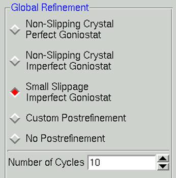
Figure 87. The global refinement options
Number of cycles. The default for the Number of Global Refinement Cycles is 10. You can change this by changing the number in the box under Global Refinement (Figure 87).
Scalepack Type. For very large or small data sets, you may need to specifically set which version of Scalepack should be used. For example, the virus version of Scalepack has memory allocations that are compatible with images that have a very high number of reflections, as would be expected for viruses of other crystals that have extremely large unit cells. In most cases, the default "Auto" option will be sufficient.
The three Scalepack output Files
The three files and their default names are output.sca, scale.out, and scale.log (Figure 88).
output.sca is the file that contains your scaled reflections. The header lists the unit cell and space group, and the five columns correspond to h, k and l, I, and σ(I). You may rename this file as you wish, although the convention is to retain the *.sca suffix to show that Scalepack created it. Many other programs that read Scalepack files expect this suffix. If you are trying to choose between space groups, it is wise to include the space group in file names.
scale.log is a log of the scaling operations. It is often quite long once the list of rejected reflections is included. You can view this file within HKL-2000 using the show logfile button.
scale.out (not visible in an Output File window) is a file that contains the data for the plots seen in the user interface. As this file is only used internally by HKL-2000, you shouldn't rename it.
The files are all written to the output data directory you specified in the Main page. However, if you fill in the path explicitly in the box provided, you can write the files anywhere you'd like.
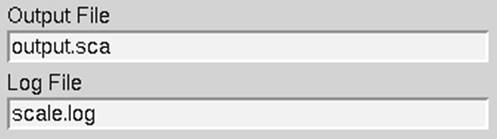
Figure 88. The Scalepack output files
|
HKL-2000 Online Manual |
||
|
Previous Integration |
Table of Contents | |