| HKL-2000 Online Manual | ||
|
Previous Scaling |
Table of Contents | |
Output Statistics and Graphs
After each round of scaling, several statistics and graphs will be displayed in the top half of the window. This section contains 1) Postrefinement statistics, 2) overall statistics, and 3) ten diagnostic graphs.
The top of the screen will have global refinement statics, including the results from post-refinement, including the unit cell parameters and information about the number of reflections (Figure 90). If you have selected the Use Auto Corrections option, more statistics will be available on the left side of the display (Figure 91). If you have selected the No Postrefinement option, only information about the reflections will be available (Figure 92).
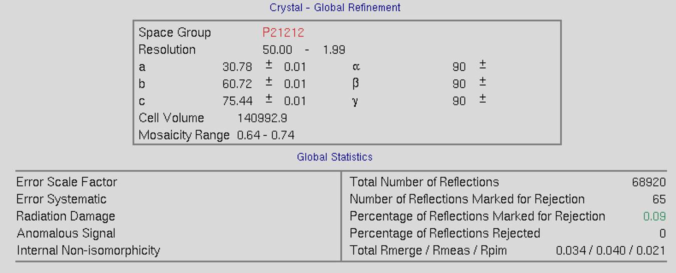
Figure 90. Global Refinement with post-refinement information
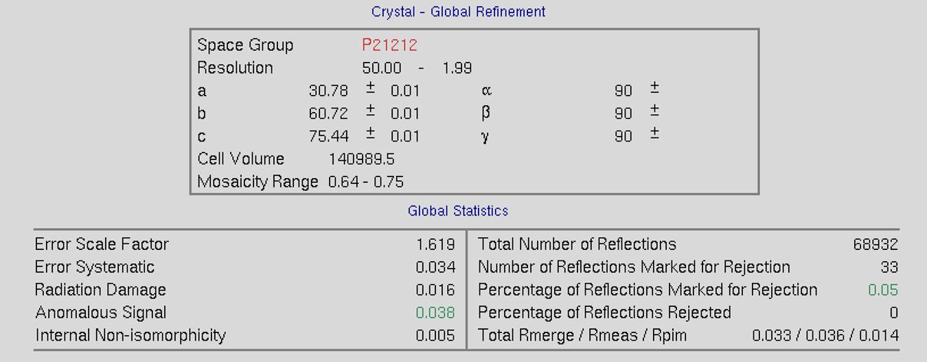
Figure 91. Global Refinement with post-refinement information and auto-corrections
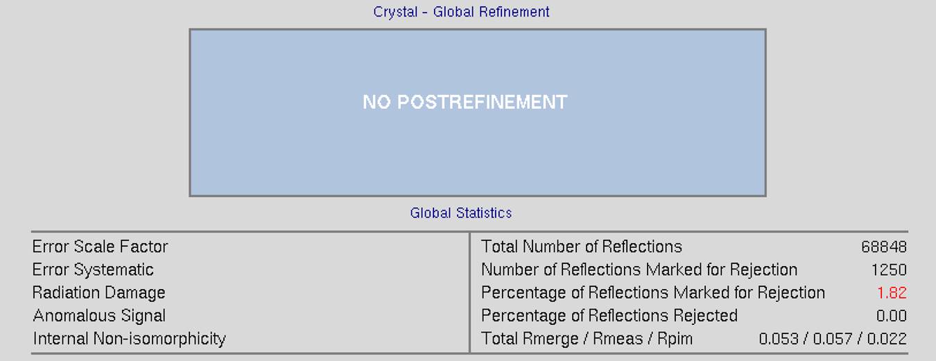
Figure 92. Global statistics with no post-refinement
Ten diagnostic graphs will appear below global refinement statistics. A scroll bar on the right allows you to view graphs that do not originally fit in the window. These graphs are:
- Scale and B vs. Frame
- Completeness vs. Resolution
- Chi2 and Rmerge vs. Frame
- Chi2 and Rmerge vs. Resolution
- I/sigma and CC1/2 vs. Resolution
- I vs. Resolution
- Chi2 and Rmerge vs. Average I
- Average and Cumulative Redundancy vs. Resolution
- Mosaicity vs. Frame
- Low-Resolution Completeness vs. Resolution
Most of the graphs have an explanation button that describes the graph. For example, the explanation for the Completeness vs. Resolution describes what the different colored lines mean (different sigma levels). Graphs that are initially displayed as logarithmic graphs also have a linear scale button that will change the scale of the Y-axis. Note that some plots have two vertical columns; in most cases, the data displayed are color-coded to match its axis. For example, blue data are plotted with respect to the blue axis and red data to the red axis. Some plots also have a button to toggle between linear and log representations.
When the initial round of scaling is finished, examine the output plots and adjust the Error Scale Factor to bring the overall χ2 down to around 1 (the overall χ2 is also explicitly specified at the end of the log file). After making changes to the Error Scale Factor, you must delete the reject file by clicking on the Delete Reject File button in the lower Controls panel, and then click scale sets again. Repeat these steps until the overall χ2 is acceptable then proceed to subsequent rounds of scaling by activating Use Rejections on Next Run and scale again. Repeat the cycle of scaling and rejecting until the number of new rejections has declined to just a few. At this point, the scaling is completed.
The first two charts can help you determine if your data collection strategy was appropriate and if the overall data collection went well. The Scale and B vs. Frame (Figure 93, right) to see if there are significant variations in intensity and B-factor of frames across the data set, which could indicate the crystal rotating out of the beam. Variations can also result from the crystal morphology. For example, plates will have more intense reflections when the crystal's edge is along the beam than when the face of the plate is perpendicular to the beam. A dramatic rise of the B-factor (to around 10) that does not decrease is usually an indication of radiation damage. The Completeness vs. Resolution plot (Figure 93, left) describes the completeness of the data for different resolution shells. The blue line represents all reflections, the purple reflections with I/σ greater than 3, the red reflections with I/σ greater then 5, the orange reflections with I/σ greater then 10, and the yellow reflections with I/σ greater than 20. This chart can be very informative for deciding if you have collected sufficient data to solve your structure. It is not necessary to achieve 100% completeness, but datasets with low completeness can severely hinder or thwart the process. Low-resolution reflections are particularly important for molecular replacement solutions.
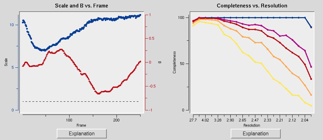
Figure 93. The Scale and B vs. Frame and the Completeness vs. Resolution and I/Sigma and CC1/2 vs. Resolution graphs
The I/Sigma and CC1/2 vs. Resolution shows the ratio of the intensity to the error of the intensity (I/σ - blue line) and the CC1/2, the correlation coefficient between intensity estimates of half data sets (upper red line), as a function of resolution (Figure 94). The traditional approach of selecting the maximum resolution was to set it to the resolution where your data falls 2σ, but recent analysis suggests that you can obtain useful information as long as the CC1/2 is above 0.2. This graph will also include an I/σ plot for anomalous data if this data is present.
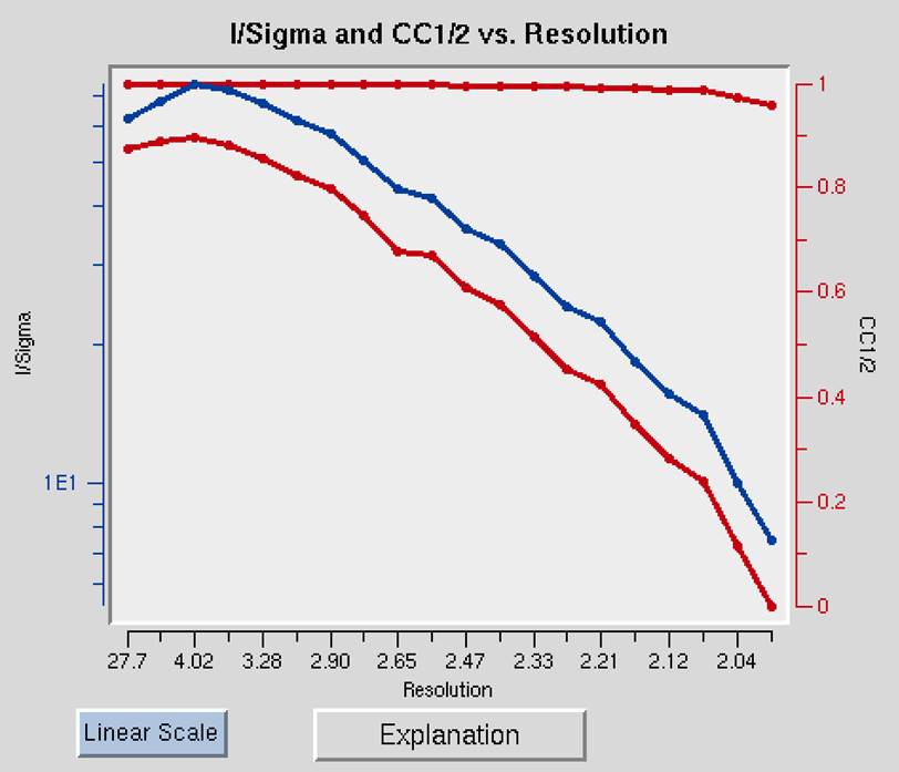
Figure 94. I/Sigma and CC1/2 vs. Resolution
Working with anomalous data
Detecting an anomalous signal is very easy. In the first step, the data are scaled and postrefined normally with the anomalous option selected (not the scale anomalous option!) This tells the program to output a *.sca file where the I+ and I- reflections are separated. In this case, Scalepack will treat the I+ data and the I- data as two separate measurements within a data set and the statistics that result from merging the two will reflect the differences between the I+ reflections and the I- reflections. Obviously, for a centric reflection, there is no I+, so the merging statistics will only reflect the non-centric reflections.
The presence of an anomalous signal is detected by examining the χ2 values on the χ2 and R-Factor vs. Resolution plot (Figure 95). The two χ2 curves show the χ2 values for each resolution shell, calculated for merged and unmerged Friedel pairs, in orange and blue respectively. Assuming that the errors scale factors were reasonable, and there is no useful anomalous signal in your data, both curves showing the χ2 resolution dependence should be flat and average around 1 when scaling with either merged or unmerged Friedel pairs. On the other hand, if χ2 > 1 and you see a clear resolution dependence of the χ2 for scaling with merged Friedel pairs (i.e., the χ2 increases as the resolution decreases), there is a strong indication of the presence of an anomalous signal. The resolution dependence allows you to determine where to cut off your resolution to calculate an anomalous difference Patterson map with an optimal signal to noise. Please note, however, that this analysis assumes that the error model is reasonable and gives you χ2 close to 1 when the anomalous signal is not present. You can only use scale anomalous when you have enough redundancy to treat the F+ and F- completely independently
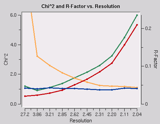
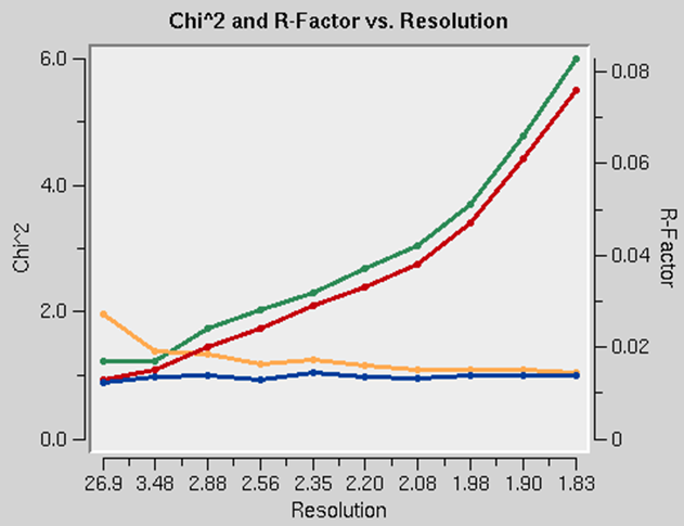
Figure 95. Anomalous signal detection for a strong (left) and moderate (right) anomalous signal.
The Scaling Controls Box
The control box in the scaling panel (Figure 96) contains the Scale Sets button, and several other options that can only be performed after at least one round of scaling has been performed.
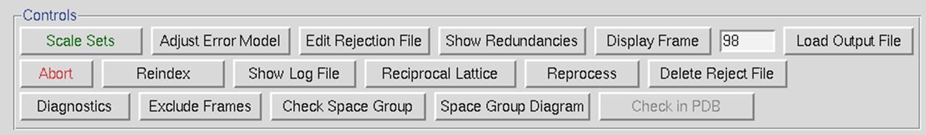
Figure 96. The Scaling Control panel
Scale Sets is the button that starts the scaling process using the parameters selected in the Scaling Options and Global Refinement boxes.
Adjust Error Model allow you to set the different error levels for each resolution shell, giving you more control over the error model than the overall effect of changing the Error Scale Factor.
The error model is the estimate of the systematic error for each of the resolution shells. There will be exactly the same number of error estimates here as there are number of zones.
The error estimates do not all have to be the same. The estimated error applies to the data which are read after this keyword, so you can apply different error scale factors to subsequent batches by repeating this input with different values. This is an important point if you enter data from a previous Scalepack output that does not need its σ to be increased.
The error estimates should be approximately equal to the R-factors for the resolution shells where statistical errors are small, namely the lower resolution shells where the data is strong. This is a crude estimate of the systematic error (to be multiplied by I) and is usually invariant with resolution. The default is 0.03 (i.e. 3%) for all zones. Examine the difference between the total error and the statistical error in the final table of statistics (this can be viewed by clicking the show logfile button and scrolling to the bottom). The difference between these numbers tells you what contribution statistical error makes to the total error (σ). If the difference is small, then reasonable changes in the estimated error values following the will not help your χ2 much. This is because the estimated errors represent your guess and/or knowledge of the contribution of the systematic error to the total error, and a small difference indicates that systematic error is not contributing much. If the difference between total and statistical error is significant, and the χ2s are far from 1, then consider adjusting the estimated error values in the affected resolution shells.
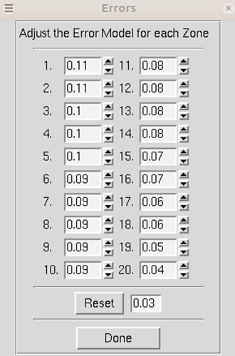
Figure 97. Adjusting the error model
Edit Rejection File will open the rejects fine in an external editor, allowing you to remove particular reflections from the list of rejected reflections. This is rarely necessary and not advised.
Show Redundancies will display a window that presents a histogram showing the percent of reflections with a specific number of redundancies. A redundancy value is the number of times a unique reflection has been measured after symmetry-related reflections have been merged. Buttons for different resolution ranges are below the histogram, allowing you to view your redundancies in different bins of data (Figure 98).
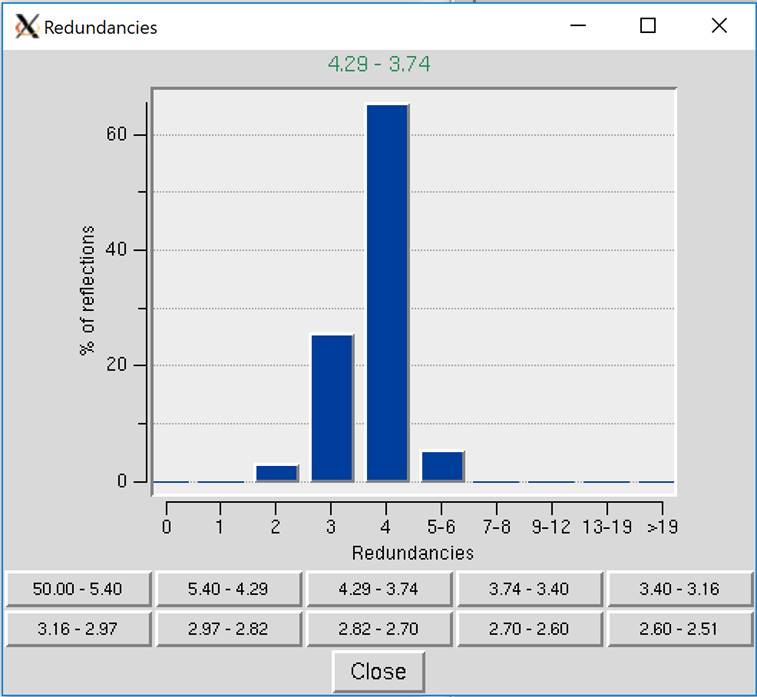
Figure 98. Redundancies Window
The Display Frame button works in conjunction with the number input box next to it. It will open the frame specified in the XDisp program.
The Load Output File will open a file selection dialog and allow you to see the output from previous scaling rounds.
The Abort button will stop the current round of scaling. This may come in handy if you realize you have set a parameter wrong.
Reindex allows you to change the reference frame for the Miller indices, effectively changing the orientation of the lattice. For example, if the data has been indexed such that a screw symmetry is on the wrong axis, you can apply a permutation to get the symmetry element on the correct axis. The Reindexing dialog lets you transpose one unit cell axis to another axis by reassigning the Miller indices. For example, if you have indexed your data in the primitive orthorhombic crystal class, the analysis of systematic abscesses may indicate that you have one screw axis. By convention, this screw axis should be on the c axis. The original indexing might have this screw axis along a different axis; therefore, you will need to reindex the data to make it conform to space group conditions.
Reindexing may also be necessary when comparing two or more data sets that were collected and processed independently. Denzo, when confronted with a choice of more than one possible indexing convention, makes a random choice. This is not a problem unless it makes a different choice for a second data set because the two will not be compatible for scaling together without first reindexing. One cannot distinguish non-equivalent alternatives without scaling the data, which is why this is not done in Denzo (i.e., at the indexing or integration step). You can tell if you need to reindex one of two data set if the χ2 values upon merging the two are very high (e.g., 50). This makes sense when you consider that scaling two or more data sets together involves comparing reflections with the same hkl or index.
To reindex the data, use the reindex button. You will be presented with different reindexing options and a manual assignment option (Figure 99). If you are working with more than one data set, you can select which datasets will be reindexed, or you can reindex all of the data sets. For example, if you have a screw axis on the b & c axes, but they should be on the a & b axes, you should select the option "abc → bca: h←k, k ←lm k←h". After choosing reindexing options, click Reindex. This example is consistent with the POINTLESS results in Figure 104.
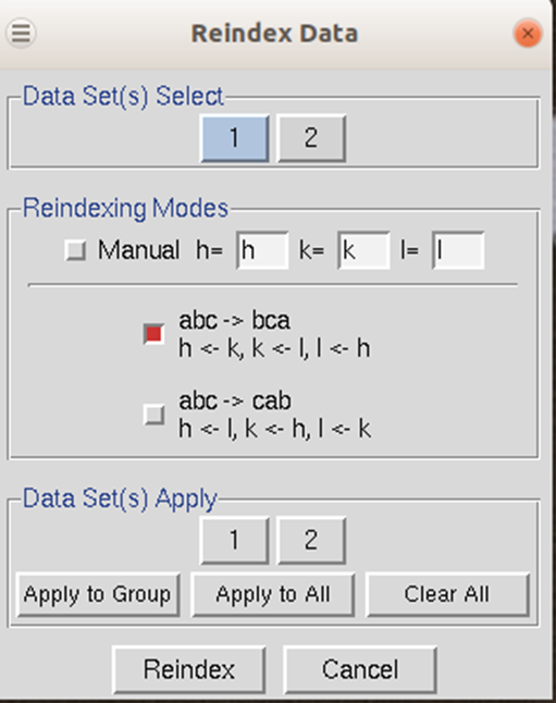
Figure 99. The Reindexing dialog
No reindexing, no new auto-indexing, and nothing except changing the sign of y scale in Denzo can change the sign of the anomalous signal.
There are two ways to manually check whether or not you have systematic absences. The first is to look at the Intensities of systematic absences table at the bottom of the log file, which can be shown using the Show Log File button. If you have scaled your data in a space group that is expected to have systematic absences, then the reflections that should be missing will be listed at the bottom of the log file. The table lists these reflections' intensity, sigma, and I/sigma. The other way to evaluate the systematic absences is to view particular slices of reciprocal space using the reciprocal lattice button.
Show Log File will open the log file that resulted from the last round of scaling. Much of the data in this file is displayed in the graphs as described below. Most of the important information is in the tables at the end of the log. The Scalepack log file can be very long since it contains the list of all *.x files read in and a record of every cycle of scaling. The log file is divided into several sections. In order these are:
1. the list of *.x files read in, and the list of reflections from each of these files that will be rejected;
2. the output file name;
3. the total number of raw reflections used before combining partial reflections;
4. the initial scale and B factors for each frame, goniostat parameters, and the space group;
5. the initial scaling procedure;
6. analysis and results tables;
7. systematic absences (if expected)
8. automatic corrections statistics (if used)
The log file should be examined after each iteration. In particular, the errors, χ2 and both R factors should be checked.
Reciprocal Lattice will open a display one of three reciprocal lattices. There are two good reasons you may want to view the reciprocal lattice: 1) If you would like to verify the space group, especially the presence of a screw axis or centering and 2) if you want to visualize the completeness of the data. Clicking the on the Reciprocal Lattice button will reveal the choice of three different slices of the reciprocal lattice to view: h,0,l; h,k,0; 0,k,l. Looking at these slices can make it apparent if you have systematic absences or, conversely, if you are missing the data necessary to determine if you have systematic absences. The h,0,l slice of the P212121 data in Figure 100 clearly shows a screw axis along h and l because the odd reflections are systematically absent.
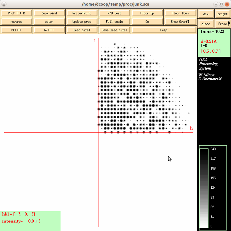
Figure 100. The reciprocal lattice viewer
Reprocess lets you take a step back and reindex all of the images using values calculated during postrefinement. You can use 1) the unit cell from prostrefinement, 2) the crystal orientation from postrefinement, and/or 3) the mosaicity from postrefinement (Figure 101). This dialog box allows you to select more than one of these parameters. This could be beneficial if there were large changes in these values as the data was initially processed. This option will overwrite your original *.x files.
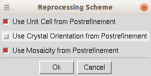
Figure 101. Reprocessing options
Delete Reject File removes the file that contains the reflections that are excluded from scaling if you have the Use rejections on next run option selected. It is important to delete the reject file if you change any of the options that affect the error model.
Diagnostics will present you with a selector panel that will allow you to run three types of diagnostics: 1) Check Integration, 2) Check Spindle Movement, and Check Shutter Timing 3). The Check Integration option will display four of the graphs generated while the data was being integrated (Figure 102). If you have more than one data set, each set will have a tab. The resulting graphs should be relatively flat. If they are not, you may benefit from the Reprocess option described above.
The Check Spindle Movement calculates the Rmerge of your data using a macro that corrects for uneven rotations of the spindle axis. This is not a common problem but does happen. If no problems are found, you should see the message "No problems with uneven spindle movement were detected." Otherwise, you will get the message, "The decrease in Rmerge indicates uneven spindle movement." You should report this type of problem to the site administrator where you collected your data.
The Check Shutter Timing calculates the Rmerge of your data using a macro that corrects for uneven shutter timings. This is not a common problem but does happen. If no problems are detected, you should see the message "No problems with synchronization between shutter and spindle axis rotation were found," otherwise you will get the message "The decrease in Rmerge indicates poor synchronization between the shutter and the spindle axis." You should report this type of problem to the site administrator where you collected your data.
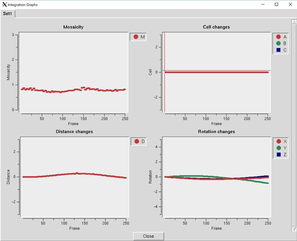
Figure 102. The Integration Graphs from the Inspect Integration option
Exclude Frames provides you with the flexibility to omit particular images from the scaling process. After integration, some frames may appear to have strong outliers in the integration information plots, like unacceptably high χ2 values i.e., far above the mean value. You can exclude those frames from scaling by clicking on the exclude frames button. A table with the list of frames will appear (Figure 103). Select a single frame by clicking on its box or on a point on the plot. Select a range of frames by checking Multiple Select and clicking twice, once on the first frame and once on the last. You may have to move to a different page with the Previous or Next buttons to see all frames. You may exclude frames above a certain limit by selecting the Select Greater Than option. This will turn on crosshairs controlled by the mouse. When you click, all frames with a χ2 higher than the horizontal crosshair. Frames marked in red will be excluded when you close the dialog and rescale. There is also an Auto Select button that will automatically select images with a χ2 higher than 10.
If you would like to see an individual frame, select the Inspect Object button, and then click on an image tile.
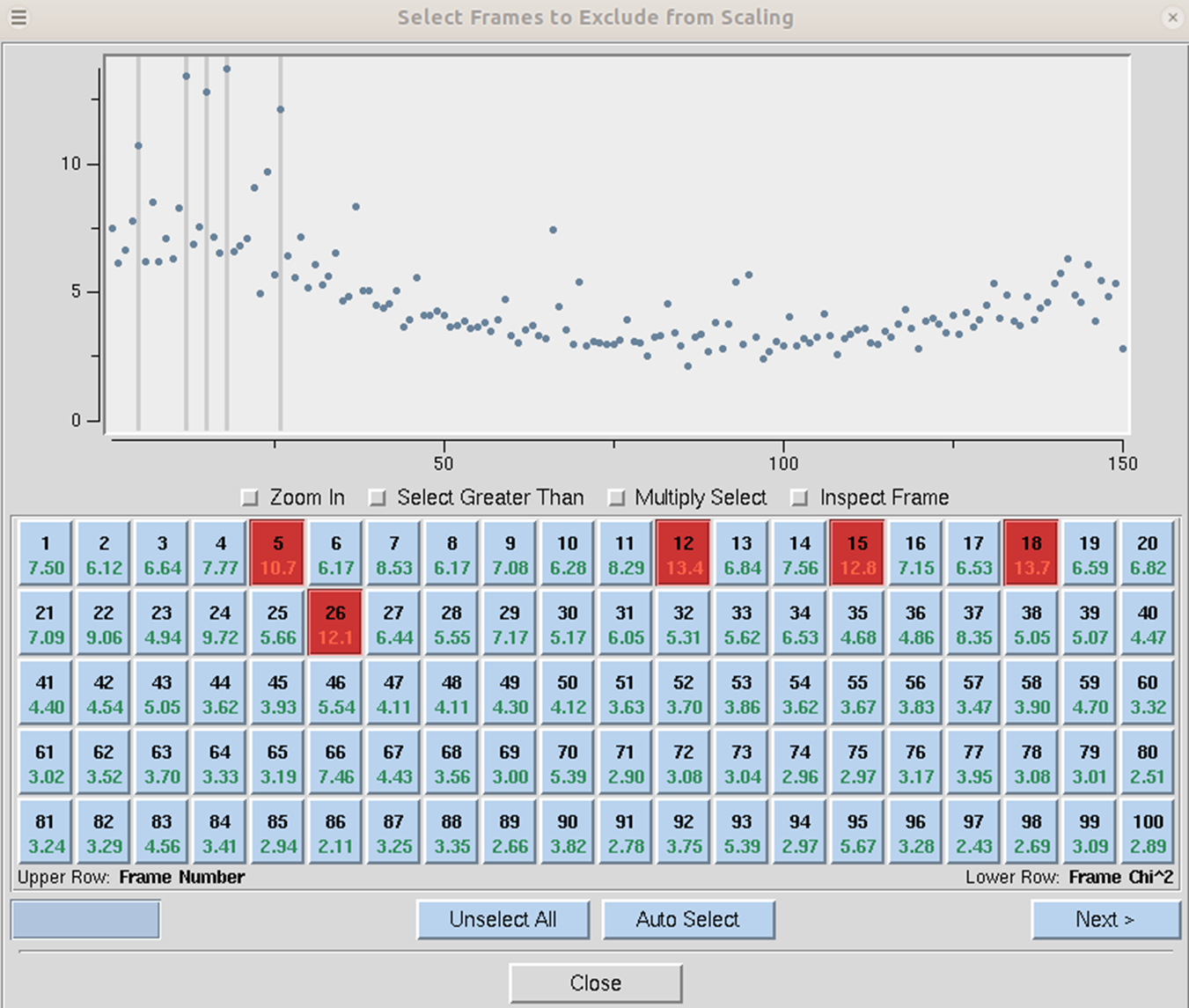
Figure 103. Frames selected to be excluded from scaling are marked red
Check Space Group and Space Group Diagram are described in detail in the next section.
Check in PDB will check the PDB to see if any deposited structures have a similar unit cell. It is unlikely, although not impossible, that two different proteins will crystallize with the same space group. This option was added to help alert you to the possibility that you have crystallized one of the proteins that have been known to co-purify with recombinant proteins, such as maltose-binding protein or trypsin.
Space Group Identification
If your installation of HKL has been linked to CCP4, then the first approach to space group determination is to use the Check Space Group button. This button runs the CCP4 program POINTLESS and will present the results in an easy to read table. To use this button, first scale the data in the primary space group for the crystal lattice (the default space group selected after integration). The dialog will not only provide the probability for each possible space group but will also indicate if re-indexing the data is necessary to ensure compatibility with space group conventions (Figure 104). The logfile from POINTLESS can be viewed. If you select the Apply button, the space group you select will be applied and put in the Space Group selection box. This will not, however, reindex your data, even if reindexing is suggested. To do this, see the section on reindexing box on page 105.
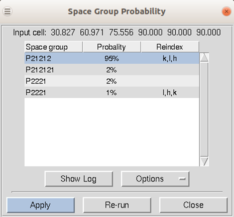
Figure 104. The Space Group Probability results from POINTLESS.
If your installation is not linked to CCP4, or if you would like to verify the suggested space group, Scalepack can be used to determine the space group of your crystal. What follows is a description of how you would continue from the lattice type given by Denzo to determine your space group. This whole analysis only applies to enantiomorphic compounds such as proteins. It does not apply to small molecules, necessarily, which may crystallize in centrosymmetric space groups. If you expect a centrosymmetric space group, you should use any space group which is a subgroup of the Laue class to which your crystal belongs. You also need enough data for this analysis to work so that you can see systematic absences.
To determine your space group using just HKL, follow these steps:
1. Determine the lattice type in Denzo.
2. Scale by the primary space group in Scalepack. The primary space groups are the first space groups in each Bravais lattice type in the table that follows this discussion. In the absence of lattice pseudosymmetries (e.g., monoclinic with β = 90°) the primary space group will not incorrectly relate symmetry related reflections. Note the χ2 statistics. Now try a higher symmetry space group (next down the list) and repeat the scaling, keeping everything else the same. If the χ2 is about the same, then you know that this is OK, and you can continue. If the χ2 are much worse, then you know that this is the wrong space group, and the previous choice was your space group. The exception is primitive hexagonal, where you should try P61 after if P3121 and P3112 fail.
3. Examine the bottom of the log file (the show logfile button) or the simulated reciprocal lattice picture (the reciprocal lattice button) for systematic absences. If this was the correct space group, all of the systemic absence reflections should be absent (or with very small values). Compare this list with the listing of reflection conditions by each of the candidate space groups. The set of absences seen in your data that corresponds to the absences characteristic of the listed space groups identifies your space group or pair of space groups. Note that you cannot do any better than this (i.e., get the handedness of screw axes) without phase information.
4. If it turns out that your space group is orthorhombic and contains one or two screw axes, you may need to reindex to align the screw axes with the standard definition. If you have one screw axis, your space group is P2221, with the screw axis along c. If you have two screw axes, then your space group is P21212, with the screw axes along a and b. If the Denzo indexing is not the same as these, then you should reindex using the reindex button.
5. So far, this is the way to index according to the conventions of the International Tables. If you prefer to use a private convention, you may have to work out your own transformations. One such transformation has been provided in the case of space groups P2 and P21.
To manually select a space group, use the drop-down box. A selection list will appear with the 14 Bravais lattices. When you click on a lattice type, it will expand to show the available space groups within that lattice type. Click on a space group to select it.
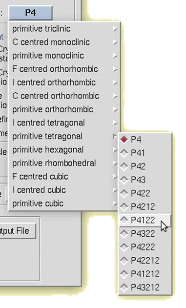
Figure 105. Manual space group selection
Bravais Lattice |
Primary assigned Space Groups |
Candidates |
Reflection Conditions along screw axes |
|
Primitive Cubic |
P213 |
195 - P23 |
|
|
|
|
198 - P213 |
(2n,0,0) |
|
|
P4132 |
207 - P432 |
|
|
|
|
208 - P4232 |
(2n,0,0) |
|
|
|
212 - P4332 |
(4n,0,0)* |
|
|
|
213 - P4132 |
(4n,0,0)* |
|
I Centered Cubic |
I213 |
197 - I23 |
* |
|
|
|
199 - I213 |
* |
|
|
I4132 |
211 - I432 |
|
|
|
|
214 - I4132 |
(4n,0,0) |
|
F Centered Cubic |
F23 |
196 - F23 |
|
|
|
F4132 |
209 - F432 |
|
|
|
|
210 - F4132 |
(2n,0,0) |
|
Primitive Rhombohedral |
R3 |
146 - R3 |
|
|
|
R32 |
155 - R32 |
|
|
Primitive Hexagonal |
P31 |
143 - P3 |
|
|
|
|
144 - P31 |
(0,0,3n)* |
|
|
|
145 - P32 |
(0,0,3n)* |
|
|
P3112 |
149 - P312 |
|
|
|
|
151 - P3112 |
(0,0,3n)* |
|
|
|
153 - P3212 |
(0,0,3n)* |
|
|
P3121 |
150 - P321 |
|
|
|
|
152 - P3121 |
(0,0,3n)* |
|
|
|
154 - P3221 |
(0,0,3n)* |
|
|
P61 |
168 - P6 |
|
|
|
|
169 - P61 |
(0,0,6n)* |
|
|
|
170 - P65 |
(0,0,6n)* |
|
|
|
171 - P62 |
(0,0,3n)** |
|
|
|
172 - P64 |
(0,0,3n)** |
|
|
|
173 - P63 |
(0,0,2n) |
|
|
P6122 |
177 - P622 |
|
|
|
|
178 - P6122 |
(0,0,6n)* |
|
|
|
179 - P6522 |
(0,0,6n)* |
|
|
|
180 - P6222 |
(0,0,3n)** |
|
|
|
181 - P6422 |
(0,0,3n)** |
|
|
|
182 - P6322 |
(0,0,2n) |
|
Primitive Tetragonal |
P41 |
75 - P4 |
|
|
|
|
76 - P41 |
(0,0,4n)* |
|
|
|
77 - P42 |
(0,0,2n) |
|
|
|
78 - P43 |
(0,0,4n)* |
|
|
P41212 |
89 - P422 |
|
|
|
|
90 - P4212 |
(0,2n,0) |
|
|
|
91 - P4122 |
(0,0,4n)* |
|
|
|
95 - P4322 |
(0,0,4n)* |
|
|
|
93 - P4222 |
(0,0,2n) |
|
|
|
94 - P42212 |
(0,0,2n),(0,2n,0) |
|
|
|
92 - P41212 |
(0,0,4n),(0,2n,0)** |
|
|
|
96 - P43212 |
(0,0,4n),(0,2n,0)** |
|
I Centered Tetragonal |
I41 |
79 - I4 |
|
|
|
|
80 - I41 |
(0,0,4n) |
|
|
I4122 |
97 - I422 |
|
|
|
|
98 - I4122 |
(0,0,4n) |
|
Primitive Orthorhombic |
P212121 |
16 - P222 |
|
|
|
|
17 - P2221 |
(0,0,2n) |
|
|
|
18 - P21212 |
(2n,0,0),(0,2n,0) |
|
|
|
19 - P212121 |
(2n,0,0),(0,2n,0), |
|
C Centered Orthorhombic |
C2221 |
20 - C2221 |
(0,0,2n) |
|
|
|
21 - C222 |
|
|
I Centered Orthorhombic |
I212121 |
23 - I222 |
* |
|
|
|
24 - I212121 |
* |
|
F Centered Orthorhombic |
F222 |
22 - F222 |
|
|
Primitive Monoclinic |
P21 |
3 - P2 |
|
|
|
|
4 - P21 |
(0,2n,0) |
|
C Centered Monoclinic |
C2 |
5 - C2 |
|
|
Primitive Triclinic |
P1 |
1 - P1 |
|
Note that for the pairs of similar candidate space groups followed by the * (or **) symbol, scaling and merging of diffraction intensities cannot resolve which member of the possible pair of space groups to which your crystal form belongs. This is inherent to crystallography.
Scaling *.x files without reintegrating diffraction images
If you have already integrated your data, you may want to rescale the data without starting from scratch, either during the same session or later on. If you have just finished processing and scaling the data, changing the output file name and changing the parameters is all that is necessary to re-scale the data in a different space group. If you are doing this to try to determine the space group, it's a good idea to put the space group in the output file (the .sca file) and the log file.
If you want to scale *.x files that you have previously processed in a new session of HKL, select scaling only when the initial site selection dialog opens, then set the Output Data Directory in the Data panel to be the directory where your *.x files are located using the directory tree. It is not necessary to set the Raw Data Directory. Next, click the Scale Sets Only button followed by load data sets. You will see a list of *.x files in the dialog box. Select the set you want to scale, followed by OK. If you want to scale additional sets of *.x files, repeat this process and add them to the list. The individual sets do not have to be in the same directory. Each set will have the file locations associated with it. Make sure the scale button is selected for each set you want to scale together. For example, if you want to scale two sets of *.x files together (say, from two different crystals, from high and low resolution passes of data collection, or from a native and a derivative, etc.) make sure that scale is clicked for each one. If you don't want them to be scaled together, then make sure that scale is not clicked. You don't have to worry about the Image Display or the Experiment Geometry since this was done when you first generated the *.x files.