|
HKL-2000 Online Manual |
||
|
Previous Project Tab After Scaling |
Table of Contents | |
Automatic Data Processing
HKL-2000 now has the ability to integrate and scale many data sets automatically. Although this process is not always successful, it has a high rate of success. This process has been tested using over 6000 datasets from the Integrated Resource for Reproducibility in Macromolecular Crystallography (http://proteindiffraction.org). Data indexing and integration were successful for 83% of the data. The correct space group was identified for 76% of the datasets.
Automatic processing uses the CCP4 program POINTLESS to identify the space group and therefore requires that CCP4 is installed and HKL is aware of the location of the CCP4 programs. CCP4 requires its own license, and the installation of CCP4 is not covered in this manual. For more information about CCP4, please see the CCP4 website (http://www.ccp4.ac.uk).
To begin the automatic processing, select the Auto tab after loading the datasets using one of the methods outlined above, using either the load data sets button on the Data tab or load a project that already has data sets you would like to process. The Auto tab will open with the set of images in the Raw Data Sets box (Figure 108). Use the Display button see the first raw diffraction image. You do not need to peek search the data. To start the automatic processing procedure, click the process button.
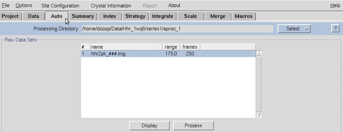
Figure 108. The Raw Data Sets window
HKL-2000 will process every file in the data set. During the first set, the word "Integrating" will flash, and the frame number being processed will update (Figure 109). This does not update for every frame, but rather is used as an indication that the process is ongoing. If the process seems to freeze, you can use the abort button to stop the process.
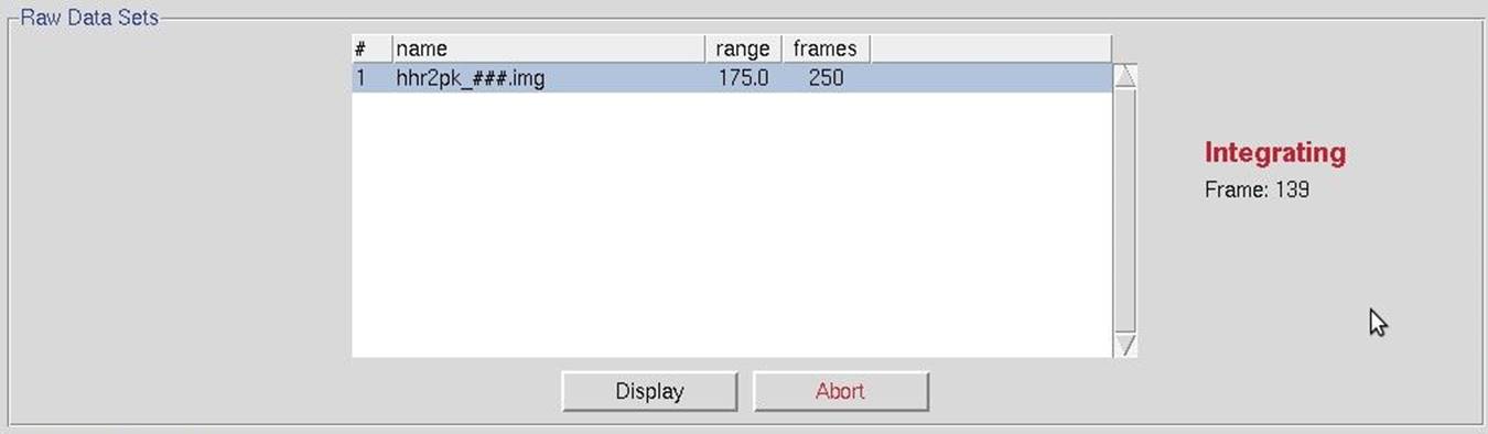
Figure 109. During automatic data processing.
Once all of the individual diffraction images have been processed, each set will be listed with some basic information about the integration process (Figure 110). The to data button can be used to create a set within the Data tab. This can be useful if you would like to manually scale the data after the process has finished. The view button will show you six diagnostic graphs about the integration process, including graphs of the frame number versus χ2, Unit Cell Changes, Normalized Number of Reflections, Changes, Distance Changes, Crystal Orientation Changes, and Mosaicity (Figure 111). These graphs should generally be flat, but some variability is OK. If you have more than one data set, the resulting graphs for each data set will be in in a different tab.
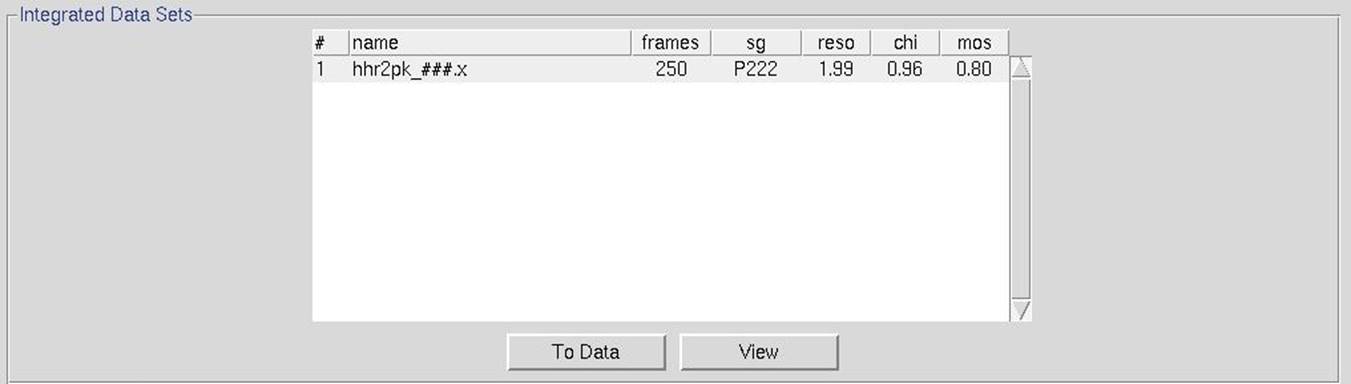
Figure 110. Automatic integration results
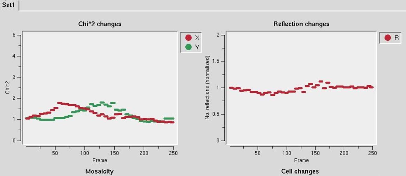
Figure 111. Automatic integration diagnostic graphs
After the integration process has finished, the reflections from all the frames need to be scaled together. During this process, the flashing word "Integrating" will change to "Scaling". Once scaling is complete, the name of the output file will appear, along with the crystals space group and the resolution chosen for scaling (Figure 112. Automatic scaling results). You can transfer this output file to the Project tab using the to project button (see The Project Tab After Scaling on page 119). The View button can be used to display the typical output from scaling (see Output Statistics and Graphs on page 97).
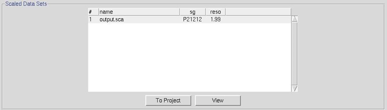
Figure 112. Automatic scaling results