|
HKL-2000 Online Manual |
||
|
Previous AutoIndexing |
Table of Contents | |
Lattice Parameter Refinement
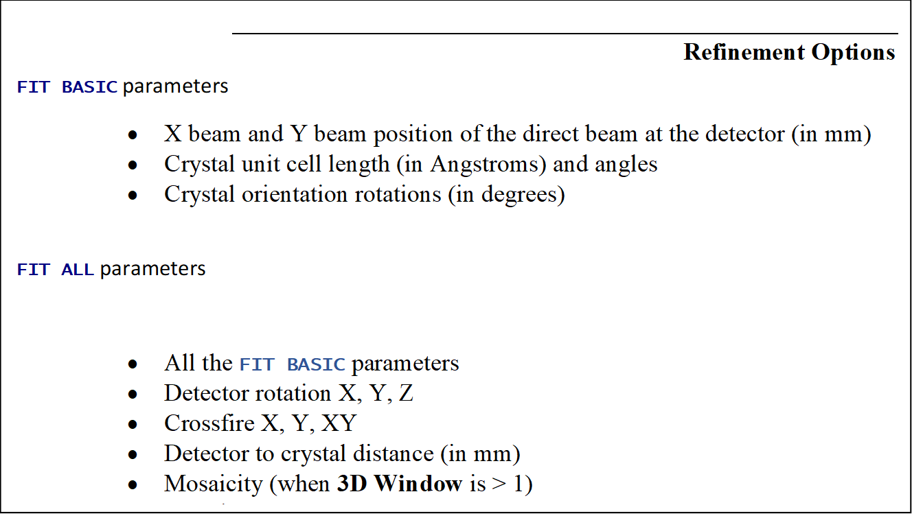
Click the refine button to refine the lattice parameters. The initial parameters are those of fit basic, and these are appropriate for auto-indexing and the first refinement step. When the Refine button is clicked, the parameters selected in the Refinement Options box (Figure 56) will be refined the number of times selected in the selector box next to the Refine button. The overall measurements of how well the selected crystal class fits the data are the Positional and Partiality Chi-Square values (Figure 57). These are also color-coded from dark green to light green to red from good to bad. The other refinement parameters that are refined are presented with their current value, how much they have changed during the refinement cycle, and the error associated with the value (from left to right). Click Refine several times, and the values should become stable.
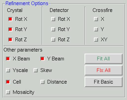
Figure 56. The Refinement Options box with the Fit Basic parameters selected
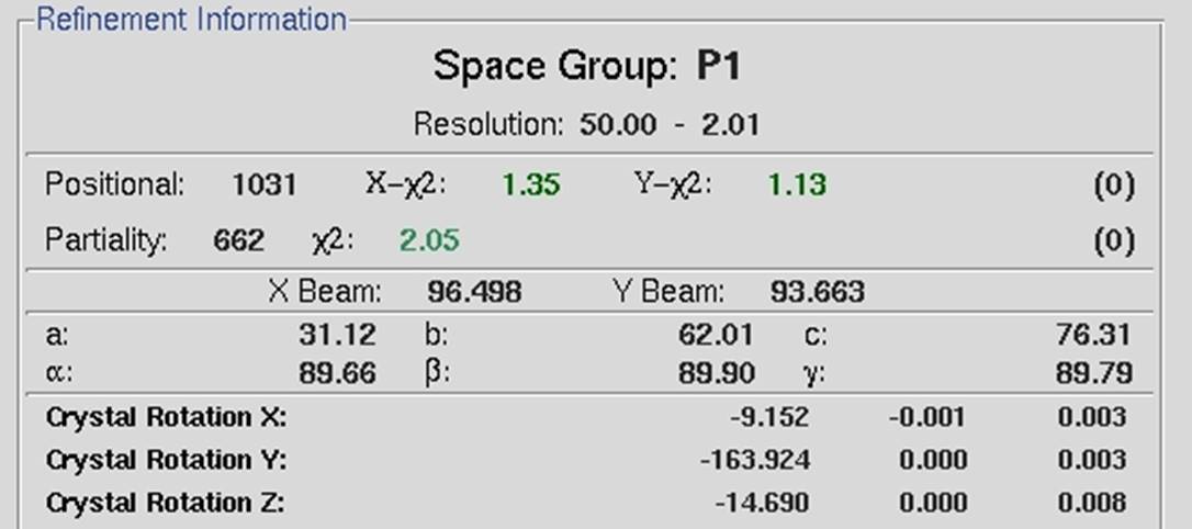
Figure 57. Refinement statistics generated using Fit Basic parameters
At this point, the predicted reflections displayed on the image are color-coded. Reflections that are recorded completely on this image will be green, whereas reflections that are split between more than one image will be yellow. These "partial" reflections will be combined during the scaling process. After a few rounds of refinement using the default parameters, check the image to make sure the predicted reflections sit on real spots. Make sure the direct beam position is correct and looks reasonable.
Click the fit all button and refine again. Click the bravais lattice button, select the appropriate lattice for your crystal, and then click the apply & close bar. HKL uses eigenvalue filtering to ensure that any parameters that are too highly correlated will be restrained by the program. The days of selective manual fitting and fixing are over. The program almost always does a better job.
When refinement goes wrong
Occasionally the auto-indexing routine does not give clear-cut results. Symptoms range from utter failure to difficulty scaling to something that is just odd. Please refer to the Trouble Shooting appendix for detailed exploration of common causes of indexing problems.
The Trouble Shooting section contains information about :
- When default settings aren't good enough
- Macros that can save the day
- Most common sources of problems
- Finding the beam position
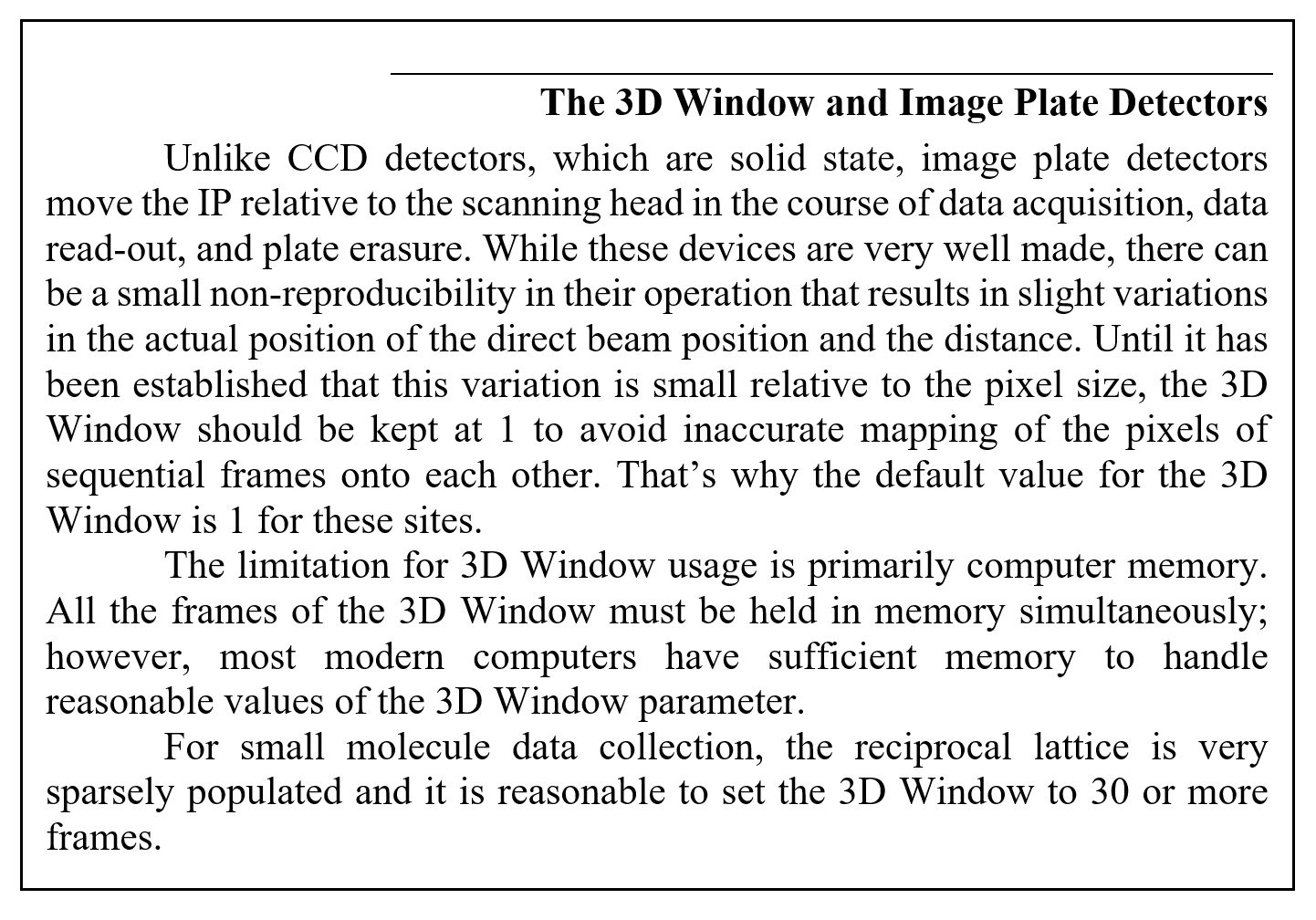
Initial 3D window setting
A good rule of thumb is to set the number of oscillation degrees covered by the 3D Window (after the resolution limits and lattice have been determined) to be at least twice the refined mosaicity. For example, if the mosaicity is about 1.0 Å, and the frame width is 0.5 Å, a value of 5 is a good choice. The default value of 5 is reasonable for macromolecular data, with a frame width of 1.0 Å. For small-molecule structure determinations, where the reciprocal lattice is sparsely populated, a 3D Window of 3-5 frames is a good choice (Figure 58).
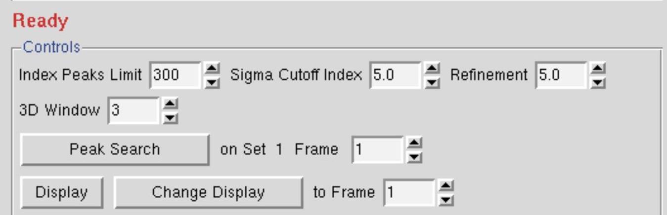
Figure 58. The 3D window in Controls box
Choosing the correct lattice
The lattice is best chosen after the first frames of the 3D Window have been refined in space group P1, but before the whole set of frames is integrated. Since primitive triclinic is the lowest possible symmetry for your crystal, if you can't succeed in refining in P1, choosing a higher symmetry lattice with less refinable parameters will be even worse.
Clicking on the refine button starts the refinement of the auto-index lattice. After auto-indexing, a small set of crystal parameters will be selected for refinement. Refine the indexing a few times using FIT BASIC, then select the FIT ALL regime; you do not want to be fixing refinement parameters. During refinement, you should notice the number of spots used in the refinement go way up, and the &chi2 errors in X and Y positions approach 1.0. Before proceeding further, go back to your diffraction Image Display window and examine the positions of the yellow or green circles with respect to the diffraction spots. If indexing and refinement worked, the predicted reflections (circles) should still match up with the diffraction pattern. If the predictions do not line up with the diffraction spots, check out the Trouble Shooting Appendix on page 137. Also consider the possibility that you are looking at reflections from more than one crystal. HKL-2000 can only predict reflections from one lattice.
Assuming that the predicted reflections still match up with the diffraction pattern and the &chi2 values are not red colored (i.e., above 5), now is the time to select the proper Bravais lattice. Click on the bravais lattice button and examine the table (Figure 59). The Bravais Lattice table shows two unit cell values for each lattice type (or three for primitive rhombohedral lattice). The top cell is a primitive cell that is close to one suitable for that lattice, and the lower cell shows the changes that need to be made to the primitive unit cell parameters (a, b, c, α, β and γ) in order to force that unit cell into each. For example, tetragonal unit cells will have all angles set to 90°. A color-coded distortion index is shown to the left of the unit cell parameter and reflects how distorted the resulting geometry is with respect to the primitive triclinic geometry. The lower the distortion index, the more likely the given lattice is correct; by definition, the distortion index for the primitive triclinic lattice is 0%. If you know (really know, not "kind of" know) the space group ahead of time, you can select the correct lattice immediately. If not, select the lattice that has the highest symmetry with a low distortion index. Once you have selected the lattice, by clicking on the little radio-button by the one you chose, click the apply button to input the new lattice. Refine the selected cell using the FIT ALL button. If the Positional and Partiality Chi-Square values do not dramatically increase, then you can assume that this is the right lattice.
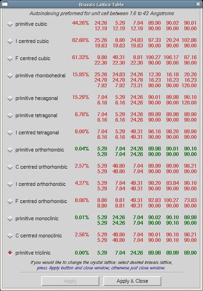
Figure 59. The Bravais Lattice table
If a lower symmetry lattice has a lower distortion index (e.g., primitive monoclinic at 0.13%) than a higher symmetry lattice (e.g., primitive tetragonal at 0.57%) then sometimes this may be the better choice, even if the higher symmetry lattice (e.g., tetragonal) is colored green. Why is this? Thanks to the use of the 3D Window in the refinement process, the indexing now uses many more reflections and encompasses a thicker slice of diffraction space than the previous incarnation of auto-indexing and refinement in Denzo. As a result, the distortion indices are much more accurate and may reflect real deviations from crystallographic symmetry, rather than just an incomplete refinement of crystal parameters.
If the highest symmetry lattice with a low distortion index does not refine well, a systematic way to choose the correct lattice is to march your way up the list of candidate lattices (candidate lattices being the green ones) and look for a significant change in the distortion index. For example, let's say you think you have a tetragonal crystal, and the candidate lattices are primitive triclinic, C-centered monoclinic, primitive monoclinic, C-centered orthorhombic, primitive orthorhombic, and primitive tetragonal. After primitive triclinic, you would select primitive monoclinic, refine, and examine the Bravais Lattice table again. The distortion index for monoclinic (and all lattices of lower symmetry - take note!) should be zero. Are the distortion indices for the higher symmetry lattices still close? If there is a significant jump (say > 0.2%) to go to a higher symmetry lattice, then perhaps those lattices are not correct, and you should stick with the lower symmetry lattice.
Keep in mind that a crystal misindexed to a lower symmetry lattice will be characterized by a high degree of "non-crystallographic" symmetry and can reliably be solved and refined as long as complete data was collected, whereas a crystal misindexed to a higher symmetry lattice will cause you no end of grief as you try to force idealized symmetry onto a system that lacks it. That's why it is important to accurately determine the lattice of your crystal early on in a data collection session, so that you will not be surprised and shocked when your best so-called "tetragonal" crystal turns out to be monoclinic, and you've only collected half a data set, and the crystal is lying in a puddle on the floor of the synchrotron hutch. Considering how fast modern synchrotrons are, you should always collect more than 180 degrees of any uncharacterized crystal, even if the indications from the first few frames make you think you have a higher symmetry crystal. However, if you suspect your symmetry is something higher than monoclinic, it is worth using the strategy prediction functionality of HKL-2000 (see Strategy and Simulation starting on page 77).
Primitive triclinic crystals
If no crystal class besides P1 is colored green, you may indeed have a triclinic lattice. For these crystals, you will have to collect 360° (go "around the world") to get a complete anomalous data set. Alternatively, your data may be misindexed (see the discussion about misindexing above and the Troubleshooting Appendix). If you are not able to see a particular pathology that would contribute to misindexing (e.g., incorrect direct beam position or incorrectly specified goniostat or detector parameters), then the best thing to do is to continue in P1 and integrate the frames. If the frames process well in P1 and the Bravais Lattice table continues to show high distortion indices for lattices other than primitive triclinic, then that is your lattice. If the frames do not process well in P1, then there is indeed something wrong with your indexing or with your data. In other words, if P1 indexes and integrates well, the lattice could be triclinic. If P1 does not index and integrate well, then the data or their processing is bad, and you cannot rule out other lattices yet. When you scale the data, you can check the space group. If you have chosen the wrong lattice, you will need to return to this step and re-index the data.
Positional and Partiality &chi2 values
The &chi2 values represent the average ratio, squared, of the error in the fitting divided by the expected error. In other words, it represents how close your observed errors are to those you predicted you would observe. &chi2 analysis is the foundation of Bayesian statistics. The numbers in parentheses are the number of overlaps for each class of reflections.
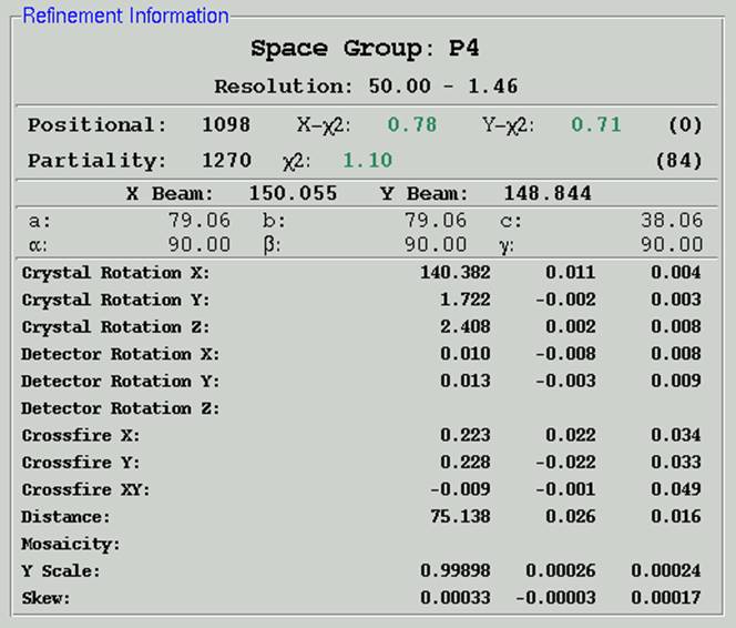
Figure 60. The refinement information using Fit All
A good refinement will have &chi2 values near 1.0. In the early stages of refinement, these values can be high, but towards the end they should be below 2 or so. All other things being equal, &chi2 values for x and y positions are sensitive to the Spot Size - a larger Spot Size will result in larger &chi2 values. Choosing a very large spot allows you considerable latitude when choosing the center of the reflection since small changes in position won't appear to have much effect on the integrated spot, and thus you will not have "pinned down" the center of the spot very well. A very small spot size, on the other hand, will be quite sensitive to the center of the reflection, since small changes here would have you integrating the sides of the reflection and not the center, and so you will detect that one place is good to be and another is worse.
The magnitude of the &chi2 values is not a critical test for the success of Denzo since they represent only the comparison of the spatial differences between the observed and predicted reflections to an error model that is typically quite strict in the prediction of small errors. Assuming default values of the error estimates, &chi2 values of 2 or even 3 are acceptable, because the position of the predicted reflection, and hence the intensity, is still very accurate. Thus, the &chi2 values may not reflect errors in the integration of the reflections.
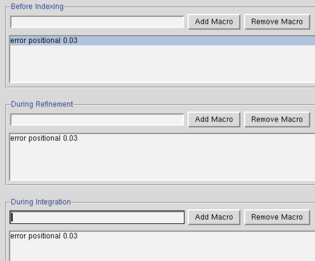
Note that you can "improve" your &chi2 values (get them closer to 1) by changing the error model. The most likely candidate for change is the value for "error positional." This value represents the error, in mm, in the positional measurement of the spot center. The default values of Error Positional are set in the program for "typical" crystal for a particular detector. This can be changed by going to the Macros tab and entering the keyword error positional [value] under the fields Before Indexing, During Refinement, and During Integration where [value] is replaced by your new error, e.g., 0.03 or 0.04 (Figure 61). Some detectors (and therefore some beamlines) will almost always benefit from using this macro.
You should be cautious about increasing the error positional value, especially for a well-tested and characterized detector, because the high &chi2 values may reflect underlying problems with your crystal, rather than an actual error with the detector. For example, your crystal may be slightly cracked, with incomplete spot splitting, and the spot shape will be enlarged and distorted, reflecting the contribution from the multiple lattices. This will lead to ambiguities in determining the centers of the diffraction spots, which will be reflected in larger &chi2 values.
It is a good idea to keep your error model roughly the same from crystal to crystal so that you can use the &chi2s to pick up any other variations in your data collection. For example, if you are getting &chi2s in the range of 2 to 5 consistently and your crystal is good, you probably have problems with detector calibration. Note that most people think that their crystals, like their children, are outstanding. At least for crystals, this is not always the case.
If the &chi2 values are very high, (> 10 or so for default values of the error parameters) something is seriously wrong with the indexing, refinement, or the detector. This will be apparent from visual inspection of the displayed image in any case.
Since the goal of Denzo is to produce a list of hkls and unscaled intensities, it does not matter that the errors in the positions differ a bit from the standard expected error. On the other hand, &chi2 values substantially different from 1 in scaling should be investigated, because this directly affects a critical result of the scaling procedure, namely the &chi2 value assigned to each scaled intensity.
Starting refinement over
To start over completely, you can go to the File menu and quit the program. However, if you just want to try auto-indexing again, you can click on the abort refinement button, go back to the image and re-do the peak search, and proceed as before. To re-set the space group without aborting the refinement, you can re-open the Bravais Lattice table and choose another lattice, like primitive triclinic. Click apply & close.
Resolution Limits, Fitting Radius, and Spot Size
While referring to the indexed image, carefully set the correct Resolution limits, Profile Fitting Radius, and Spot Size. Click the refine button to update the display after changing any of these parameters. If the Crystal Rotation Y value displayed in the Refinement Information panel is colored red (i.e., for 45o < Crystal Rotation Y < 135o) click on the reference zone button in the Controls panel and choose a new zone with a better value for roty.
The Profile Fitting Radius
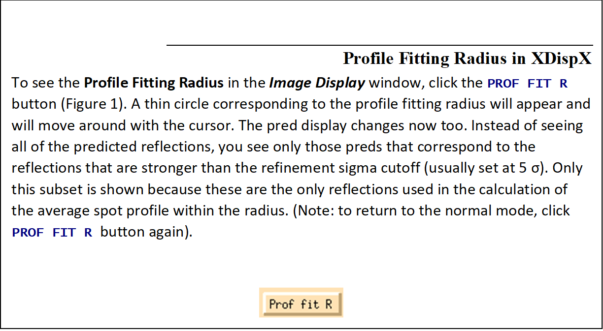
The Profile Fitting Radius is the radius of the area around each particular spot, in mm, containing neighboring spots, used to calculate the average spot profile (Figure 63). The spot in question is fitted to the average profile of all the spots within the specified radius. Generally, the radius is set so those spots on roughly 3-5% of the area of the detector are included in the averaging. You can display the profile fitting circle using the Prof Fit R button
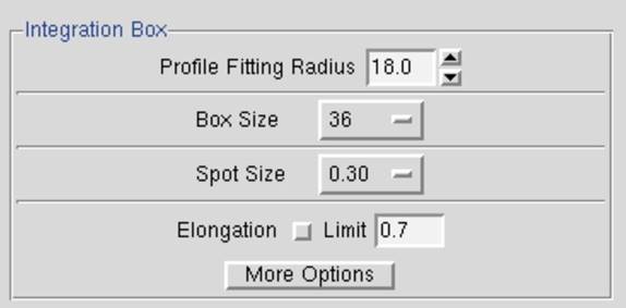
Figure 62 The Profile Fitting Radius is set in the Integration Box
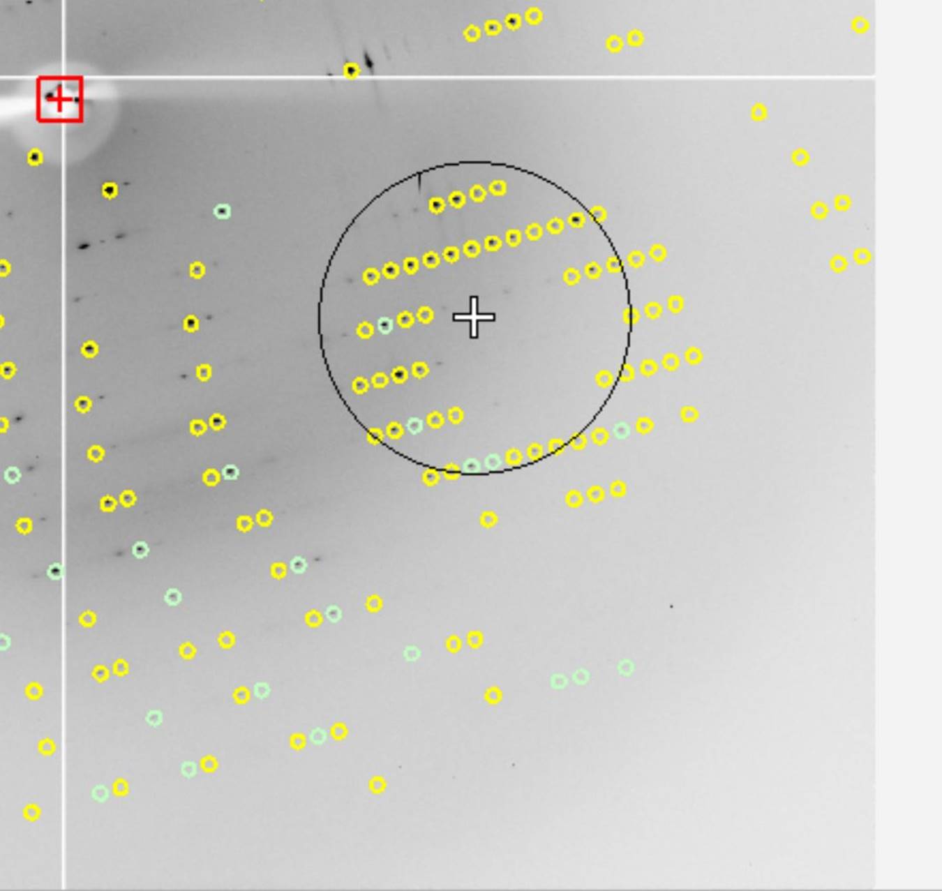
Figure 63. The profile fitting radius can be displayed and moved around.
The particular size of the area chosen depends on how much the profiles vary across the film and the density of the spots on the film. For example, if the spot profiles vary a lot across the film, then you would choose a smaller radius. If you have a small lattice and the spots are widely separated, you might want to choose a larger radius.
The calculation of the average profile is a time-consuming task, and it is proportional to the number of spots in the profile fitting radius circle, but too small a radius will not capture enough spots and lead to a noisy average profile. Too large a radius will average out significant profile variations.
A good rule of thumb is that the Profile Fitting Radius should enclose about 10 to 50 spots whose intensities are above the weak level. Useful increments of the profile fitting radius are 2.5% of the detector size (e.g., 5 mm for a 200 mm wide IP).
The profile fitting radius can be set in the Index window under the Integration Box panel in the lower-left quadrant of the window (Figure 63). The value is given in millimeters, and you can adjust it iteratively, hitting the refine button in between your guesses. In general, it is preferable to enlarge the radius to make sure that there are no orphan reflections (reflections that, when placed in the center of the circle, have no other non-weak reflections within the circle). However, keep in mind that if you are using a 3D Window greater than 1, that the Profile Fitting Radius is actually the "Profile Fitting Sausage," since it encompasses the stack of frames in the 3D Window, and more spots may be used than first seems from examining a single frame.
Setting the Spot Size
The final parameter to set is the Spot Size. This is generally a function of the size of your crystal and the quality of the X-ray beam (collimation, crossfire, parallelism, etc.), but it must be set for proper integration. Each reflection can be thought of as a buffered region (usually a circle) within a box. As seen in Figure 65, each reflection can be divided into three different regions. Here, the light blue region is the background region, and the measured reflection is in the unshaded region in the center. The dark blue region is a guard region, which is not used to calculate either the reflection or the background. The yellow circle is the predicted position of the reflection. Its size is not used in calculations.
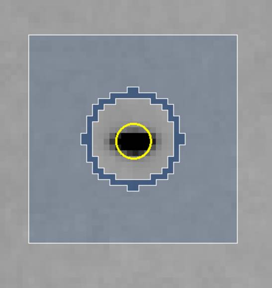
Figure 65. A Single Reflection
If you choose too small a Spot Size, significant data is lost because the reflections will be rejected because of the reflections extending into the background region. Choosing too large a Spot Size runs the risk of 1) rejecting reflections due to overlaps, 2) including portions of the neighboring reflection in the measured intensity, and 3) including too much of the background in your intensity measurement.
Setting the Spot Size is somewhat of a tradeoff, since not all the spots on an image are of the same size, and one spot size and shape must suffice for the entire set of images (with the exception of correcting for the elongation caused by the intersection of reflections at high angle to the detector face, which is corrected by the parameter Elongation Limit). However, it is unlikely that your data will suffer too much because profile fitting limits the damage caused by including the background in the spot. As a general rule of thumb, it is best to try to adjust the spot shape to fit some of the medium to strong spots on the image.
The spot can be either circular or elliptical. Clicking on the more options button gives you more control of the spot and background limits. You also have the option of defining elliptical spots if your spot shapes are sufficiently elongated (Figure 66).
After making the changes to your spot shape, or turning on the Elongation Limit option, you can verify that the spot shape has changed by examining the image and the predicted spots in the Zoom window of the Image Display window (you may have to click update pred to show the predictions).
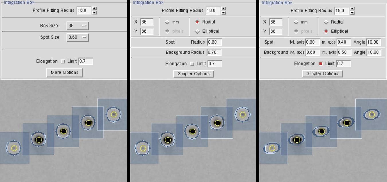
Figure 66. The Integration Box and Zoom windows are shown with simple options (left), radial options (center), and elliptical options (right).
What is the Elongation Limit?
Note that Denzo now has an option to take into account the radial elongation of the spots that arise from the intersection of the diffracted X-rays at a high angle with the detector. This is activated by checking the Elongation Limit button in the Integration Box panel. The default value for Elongation Limit (expressed as the fraction of the box size the spot is allowed to elongate) is 0.7. The range is from 0 to 1.
Setting the integration resolution limit
Examine the indexed diffraction pattern carefully. T[DRC2] [DRC3] he cursor can be used to determine the resolution of a particular spot. In general, you want to be on the generous side (say 0.2 °) with setting the resolution limits, since they can always be lowered in Scaling if you were too optimistic. Conversely, if you are too stingy with the resolution limits in Denzo, you will have to go back and re-integrate all your frames again since Scalepack cannot increase the resolution limits beyond what you have set in Denzo. You may have to darken the image using the histogram slider to see the high-resolution reflections clearly. Using the Zoom function also helps. Once you have determined the proper resolution limits, go back to the Index window and input the new resolution limits into the proper box. Then hit the refine button again, and the new predicted reflections will appear in the diffraction pattern window. You may have to do this a couple of times until you get it right. Look in all quadrants of the diffraction image, (and if possible, multiple frames) as crystals often diffract anisotropically.
Another feature that you can use to estimate the resolution of your data is the predicted reflection circles. By default, reflections that are above the sigma cutoff for indexing will be displayed. If you set this limit to 2 sigma, you can get a good feel for the resolution you can get by checking the resolution of the reflections closest to the edge (or corner). You can also compare the predicted reflections above the sigma cutoff with all predictions to get a feel for the fraction of reflections above the cutoff limit. To toggle which reflections are shown, use the selector found next to the prediction toggle button. As mentioned above, it is good practice to process the diffraction images to a resolution that is slightly better than you think your ultimate resolution.
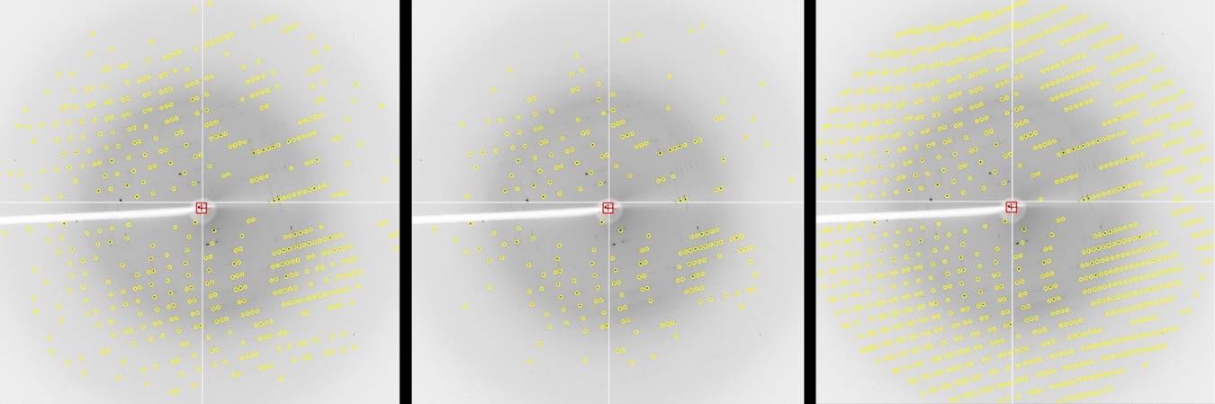
Figure 67. Predicted reflections at 2 sigma, 20 sigma, and all reflections.
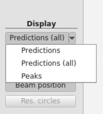
Figure 68 The Prediction selector
One more thing you can do to get a feel for the resolution of your diffraction is to display the resolution circles. Found in the resolution dialog box, you can set the resolution of five circles to display (Figure 69). These can be toggled on and off using the Res Circles button.
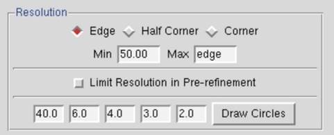
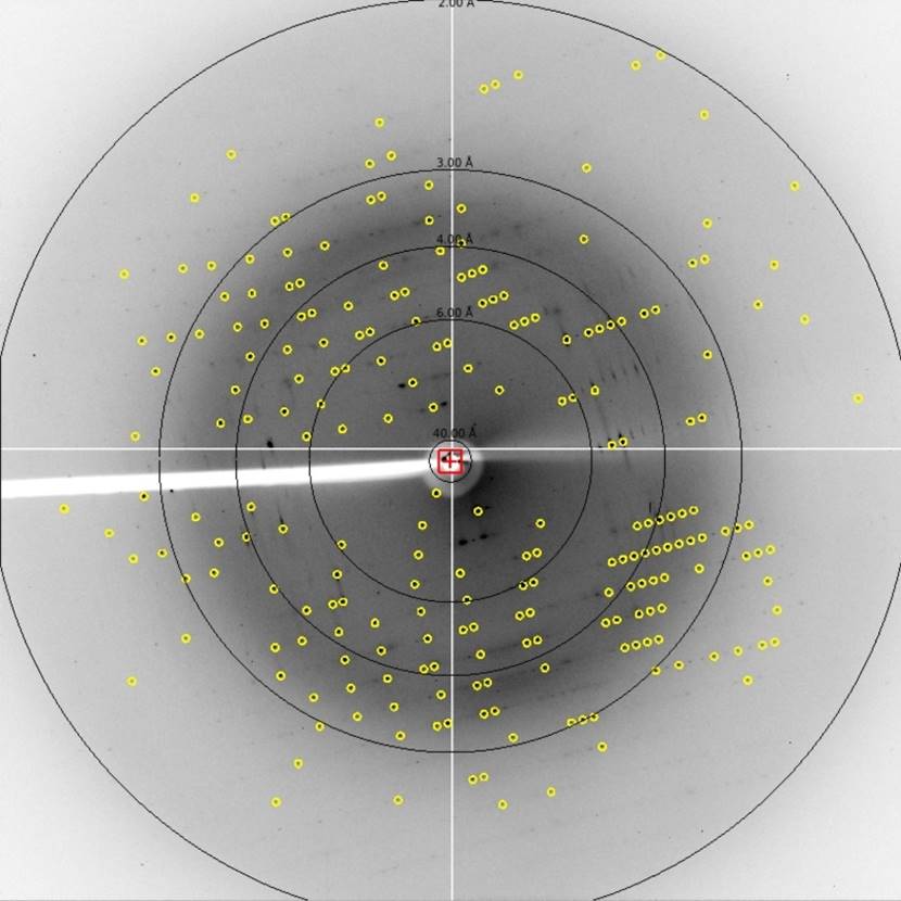
Figure 69. Resolution circles dialog and the displayed circles.
The Crystal Rotation X, Crystal Rotation Y, and Crystal Rotation Z parameters
The crystal Crystal Rotation X, Crystal Rotation Y, and Crystal Rotation Z angles define the orientation of the crystal lattice in space for the calculation of the predicted reflections. It is inconvenient and non-intuitive to work with images in the data conventions because we are used to thinking about diffraction geometry in terms of the X-ray beam, the spindle axis, and the laboratory frame of reference (horizontal, vertical). There are two possible conventions within this "intuitive" set:
Gravity/beam system (used in XDisp, but not used in Denzo)
In this system, the X-ray beam is defined as being perpendicular to the direction of the force vector due to gravity ("down"). The beam is the z axis, gravity is parallel to the y axis, and the x axis is perpendicular to both of these. In terms of crystal orientation rotations
n Crystal Rotation Z would denote rotations or the crystal around the beam axis,
n Crystal Rotation Y would denote rotations of the crystal about the vertical axis
n Crystal Rotation X would denote rotations of the crystal about the horizontal axis.
This convention has the advantage that it does not change with different camera spindle geometry. In addition, it corresponds directly to the common orthogonal detector directions, in that the detector directions x and y on the film or IP are perpendicular to the X-ray beam. A disadvantage of this system is that the x axis may or may not correspond to the spindle axis, depending upon the &chi (chi) and ω (omega) setting angles of the 3-axis goniostat. For the purposes of aligning your crystal, this makes life more complicated, as we are used to thinking about aligning crystals by moving the arcs on a goniometer head. For &chi equal 90 or 270 degrees and ω equal to zero. However, the spindle axis is parallel to the x axis, and thus Crystal Rotation X corresponds to rotations about the spindle axis.
Although this system will not (formally) work in outer space (where the gravity vector is essentially zero), nor in the event that the X-ray beam is vertical, the fact remains that (so far) all macromolecular crystallography is done with horizontal X-ray beams on the surface of good old planet Earth, and thus it is a viable option. While Denzo does not use this convention, XDisp does.
Spindle/beam system (used in Denzo)
The spindle/beam system is the Denzo crystal and cassette orientation convention. In this system,
the z axis is again parallel to the beam,
the x axis is parallel to the spindle axis and
the y axis, also termed the "vertical" axis (for want of a better word), is perpendicular to the spindle and beam axes.
In terms of crystal orientation rotations:
Crystal Rotation Z would again denote rotations of the crystal around the beam axis,
Crystal Rotation X would denote rotations of the crystal about the spindle axis and
Crystal Rotation Y would denote rotations about the axis perpendicular to the beam and the spindle.
The advantage of this system is that it is very intuitive to the crystallographer. In addition, with Eulerian &chi values of 0, 90, 180 or 270 degrees the spindle and vertical axes are parallel to the x or y axes of the detector. The main disadvantage of this system is that it is dependent on knowing the geometry of the camera.
While the crystal and cassette orientations follow the spindle/beam convention for Denzo, the beam, boxprintout, spot, margin, film width and length in the Denzo log file follow the data convention.
The X-beam and Y-beam values are the distance from the edge of the detector data collection area to the beam spot, in mm. These are perhaps the most important parameters.
Crossfire is a measure of the X-ray beam divergence and focusing as it leaves the collimator and illuminates the crystal. Crossfire, being a symmetric tensor, has x, y, and xy components. It affects the prediction of partial reflections and their positions, not their angular width. It is expressed as angular divergence of the beam. The default value is zero crossfire, i.e., a perfectly parallel beam or a beam focused on the detector.
The Reference Zone
The Reference Zone shows the current zone and other zones which are crystallographically equivalent to the current zone. Keep in mind that upon indexing the crystal for the first time (which is just another way of stating that the crystal orientation parameters are being determined) Denzo makes an arbitrary choice of reference zone (Figure 70). Being able to choose an equivalent zone is useful in a number of ways.
1. If the crystal Crystal Rotation Y happens to fall between 45 and 135 degrees, the refinement of the crystal orientation is more difficult for the underlying algorithm (although it will still work). Choosing an equivalent zone from the list is an easy way to overcome this. Change the reference zone if the Crystal Rotation Y parameter is colored red.
2. If two or more data sets are collected from the same crystal, without removing the crystal or changing its orientation relative to the goniostat, and the data sets are indexed independently of one another, then it is possible that Denzo will arbitrarily assign a different reference zone to the two data sets. Unfortunately, this will result in a different original index for reflections which otherwise should be equivalent, and so merging reflections between data sets will not work. However, by choosing the same reference zone for both data sets, scaling and merging reflections can be done correctly and accurately.
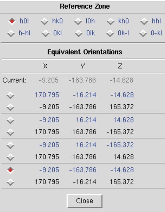
Figure 70. The Reference Zone window
The 3D Window and Mosaicity
The 3D Window specifies the number of consecutive frames from which the reflections will be integrated simultaneously. Set the 3D Window so that the oscillation range encompassed by this sector of reciprocal space is at least twice as large as the refined mosaicity. Typically for CCD data, five frames are used, but if small oscillation angles are used, then this value will need to be increased. One principal advantage of the 3D window is that binning frames together can include more reflections in the refinement, thereby increasing the accuracy of indexing on frames that have very few reflections (e.g., small molecule data sets, low mosaicity / small unit cell macromolecular data sets, low-resolution macromolecular data sets). The disadvantage of grouping frames together is that local variations in frames are averaged out (e.g., "bad" frames, frames where the crystal slipped, etc.)
Mosaicity is defined in Denzo as the rocking angle, in degrees, in both the vertical and the horizontal directions, which would generate all the spots seen on a still diffraction photograph. It not only includes contributions due to X-ray bandwidth, beam crossfire, etc. but is also a characteristic of the crystal itself. Mosaicity is refinable when integrating your frames if the 3D Window is set to be at least twice as large as the refined mosaicity. For example, if your crystal has a mosaicity of about 1 Å, then a 3D Window encompassing 2 Å or more of data should allow for proper refinement.
The best way to set the mosaicity is to use the 3D Window and let Denzo refine it in the course of integrating the reflections. If you are unable to use a 3D Window greater than 1, and the mosaicity is greater than half your oscillation range (which is usually the case), then you will have to set the mosaicity manually. You do this by going to the Crystal Information button and entering the Mosaicity in the field provided. If you have to do this, remember to uncheck Mosaicity in the Refinement Options.
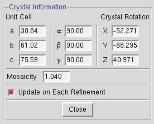
Figure 71. The Crystal Information window
A correctly set mosaicity will not always result in predictions covering all of the reflections on an image. In particular, very strong low order reflections may require unreasonably large values of the mosaicity for coverage. These reflections may not represent the intrinsic mosaic spread of the crystal, but rather may result from particularly intense diffraction from that lattice point. A mosaicity that is set too high is usually better than one that is set too low, but setting the mosaicity too high could result in an unnecessarily high number of overlaps.
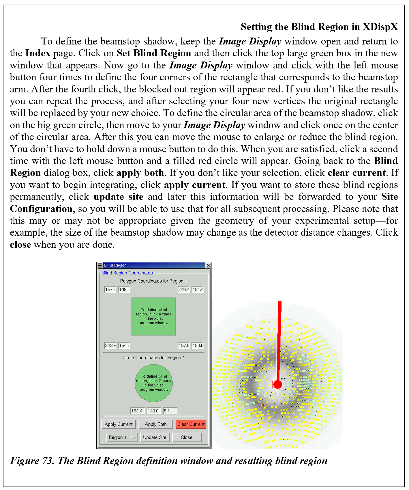
Masking the beamstop and other shadows
It is important to define the area of the beamstop shadow. If the beamstop shadow region is not defined explicitly, Denzo may fail under certain circumstances of high background to reject potential reflections, which are obscured by the beamstop. These few inaccurately measured "reflections" will severely degrade the quality of your anomalous signal. XDispQt allows you to set two distinct blind regions and two shadow regions. Shadow regions are regions where diffraction is not completely blocked, but the background and overall intensity is lower than the rest of the image. This can result from X-rays being blocked by the goniometer. The background will be treated differently in shadow regions.
To open the Masks dialog, click the Edit Masks button on the left of the display. The dialog (Figure 72) allows you to set to polygon and circular region for each blind region or shadow region. Polygons will be shown with red circles at the vertices, that can be grabbed and moved with the mouse (or stylus). Circular masks have one red circle that is used to set the radius of the mask. Both types of masks can be moved with a click-and-drag motion of the mouse. You can select with which mask to work with by either clicking on the corresponding button in the mask dialog or by clicking within the mask you want to work with. A mask can be removed by selecting it, then clicking on remove in the dialog. If you have more than one mask or shadow region, the polygon and circular region will be color coordinated. When you are finished working with the masks, click finish on the bottom left to remove the mask dialog and return to the normal viewing mode. The mask regions will not be displayed in the normal viewing mode, but the information about the masks will update the site configuration dialog. The masks you set will be used during your current HKL session. If you want to save this information to the site definition, click save site info in the site configuration dialog.
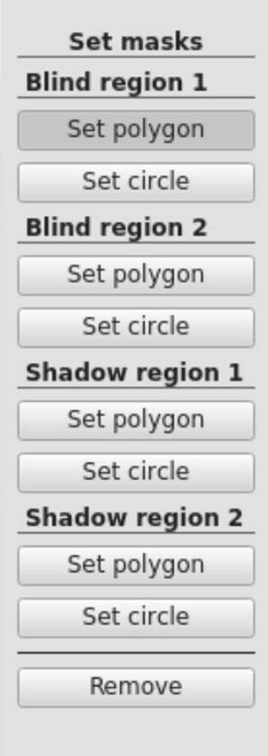
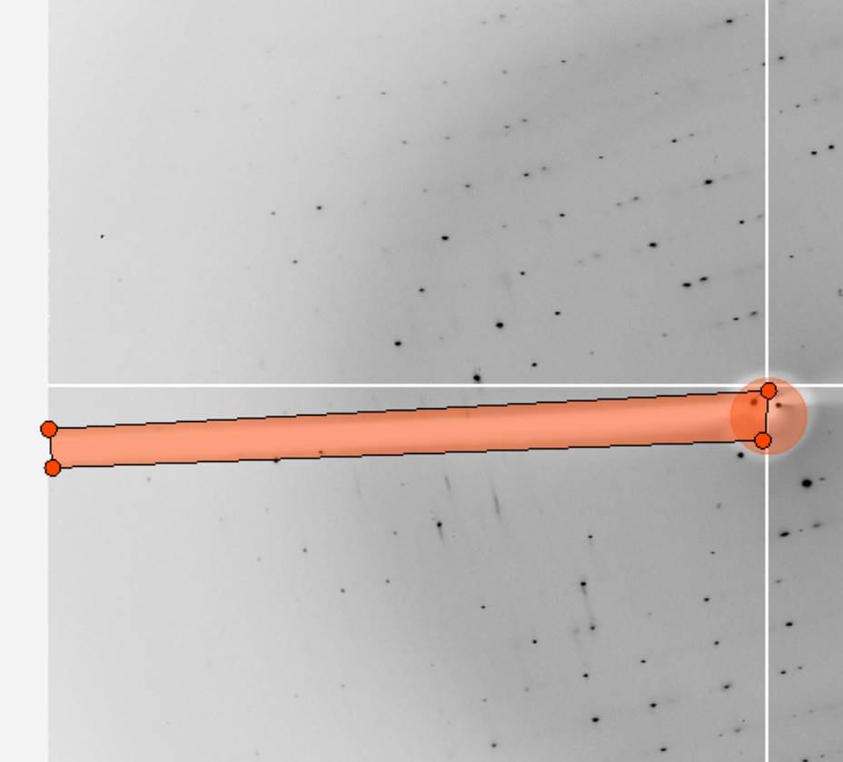
Figure 72. The Mask dialog (left) and setting the polygon of Bling region 1 (right)
|
HKL-2000 Online Manual |
||
|
Previous AutoIndexing |
Table of Contents | |