|
HKL-2000 Online Manual |
||
|
Previous Lattice Parameter Refinement |
Table of Contents | |
Strategy and Simulation
Strategy
Data collection is not an automatic process. In a perfect world, crystals would be perfect and have negligible mosaicity, crystal lifetime would be unlimited, crystal exposures would be short, data collection time would be unlimited, and disk storage capacity would be infinite. In this case, one would just choose a tiny oscillation range and collect 360 degrees of data without worrying about the consequences. However, as we all know, crystals are imperfect and decay fast, data collection time is not unlimited, and storage space is not infinite. Thus, we have to make strategic decisions about how we will go about collecting a diffraction data set to avoid having an incomplete data set or one that is ruined by overlapped spots. This involves making decisions about the oscillation range to collect, the width of each frame, and the exposure time per frame. The strategy and simulation utilities in HKL-2000 can help you determine an optimal data collection strategy.
In order to calculate a strategy, you first need to collect and index a few frames. The strategy module will work with just one frame but will work better if a few frames are available due to the increased accuracy of the mosaicity calculation. Index a frame or set of frames as usual, making sure that the correct Bravais lattice is selected, the resolution is properly chosen, and refine with the fit all regime (including mosaicity with the use of 3D window). Do not proceed to the integration step.
Once the first frames are indexed, click on the Strategy tab. This tab is divided into three regions. Three control boxes are on the left: space group, strategy, and simulation. On the right, there are four initially empty chart areas. The top two are the Strategy and Simulation charts. A scroll bar on the right is necessary to see the remaining charts, Completeness vs. Resolution, and Average and Cumulative Redundancy vs. Resolution. The control box at the bottom of the screen is used to combine the results of different simulations (Figure 74).
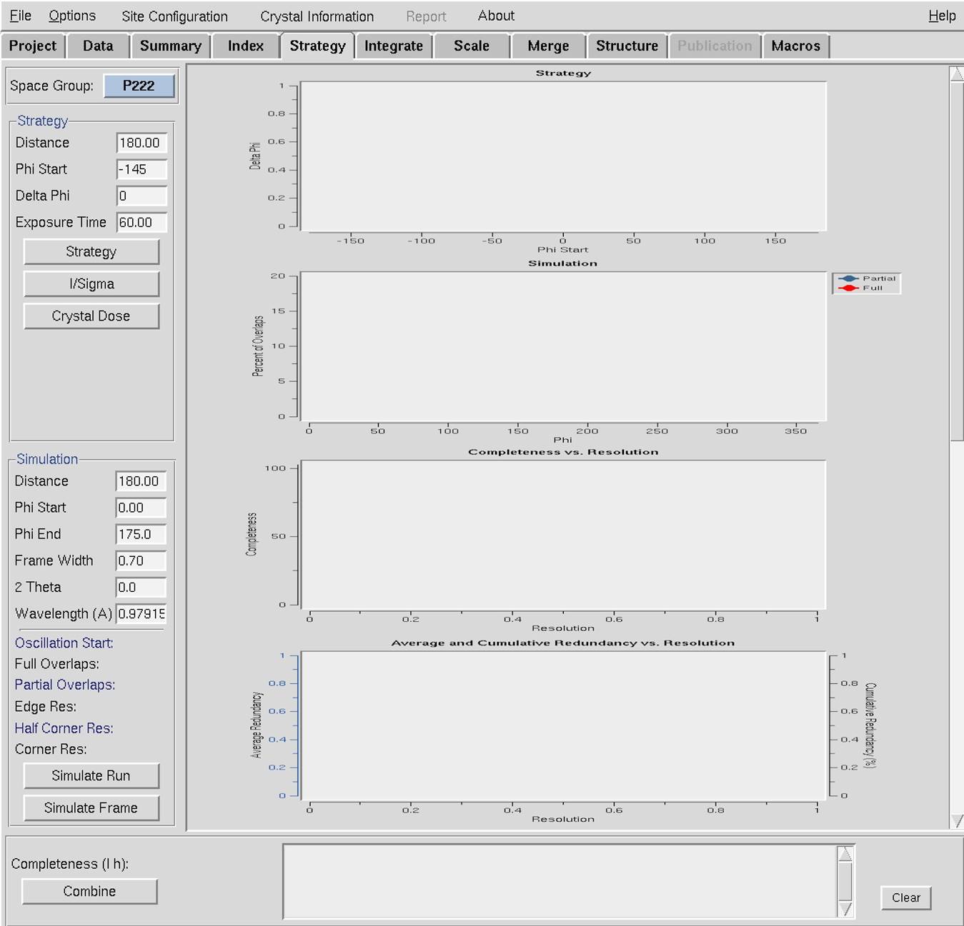
Figure 74. The blank Strategy tab (chart areas compressed to show them all).
By default, the space group of the Bravais lattice will be selected in the Space Group control window, and the parameters of the strategy window will correspond to the values of the frames that have been indexed.
Start the strategy prediction with the strategy button. In a few seconds you will see a series of colored lines in the Strategy plot, which shows the number of degrees of data you would have to collect to achieve specific levels of completeness by charting Delta Omega vs. Omega Start, or depending on the goniostat, the rotation angle (Kappa, Chi, Phi) used for the oscillation (Figure 75). The different lines indicate various levels of completeness, with a color key indicated on the right. At a given Omega (Kappa, Chi, Phi) Start, the value of Delta Omega for each line is the number of degrees of Omega you have to collect starting at Omega Start to get the percent completeness represented by the line. In other words, each line corresponds to the percentage of a complete data set that can be collected for a chosen starting oscillation angle (Omega Start) and the total number of degrees collected (Delta Omega).
Thus, considering the example in Figure 75, if only a 20% complete (dark blue line) data set is desired (although why you'd want that is somewhat mystifying), only a 6° wide oscillation needs to be collected, regardless of starting angle. On the other hand, most people want > 95% complete data sets, so the lines toward the top of the chart are more relevant. The triangular gray region present in Figure 75 marks the region that is not available for data collection. Usually, these regions are inaccessible due to limits set by beamline staff or by hardware limitations. Sometimes at home sources, it is possible to rotate into these regions, but doing so could cause damage to the detector and should be avoided.
Without clicking the mouse, move it around in the window, and a crosshair will appear. Let say you want to collect a 100% complete data set. Line the crosshairs up on the line corresponding to 100% complete. As you move it around, notice that the Omega Start and Delta Omega values in the control box are updated. To use and collect a complete data set with the smallest possible oscillation range, choose a point on the 100% line at an Omega Start value where the Delta Omega is at a minimum.
Note that for most high symmetry space groups the plots will resemble a sawtooth with a rapidly rising leading (left-hand side) edge. This jagged shape is a result of the symmetry. As you rotate a crystal in a beam, it is possible to collect some data, then collect some symmetry-related data before collecting more unique data. It is better to err slightly on the side of caution and select an Omega Start value a few degrees less than the point with the minimum Delta Omega, to avoid the high side of the sawtooth. If you do not have a high symmetry space group, the plot will look more like a horizontal line or a gentle wave. In those cases, there is not much strategy to ponder, since the lattice does not allow for much economy in data collection. Just be sure to select a strategy that does not venture into the inaccessible region.
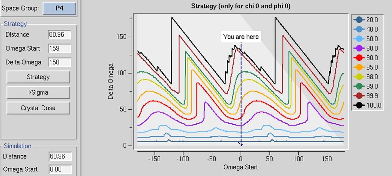
Figure 75. The Delta Omega vs. Omega Start plot
Once you have settled on a Delta Omega and Omega Start point on the plot, click the mouse and the values will be entered into the appropriate boxes in the Simulation control panel.
The I/Sigma and Crystal Dose buttons
You need to collect at least 3 frames to use the i/sigma button, and the program will estimate (after a quick integration and scaling) I/σ up to the resolution value at the edge of the detector for the specified detector distance. A new window Current I/Sigma opens with an I/Sigma vs. Resolution plot (Figure 76). Two gray lines are drawn on the plot, at I/σ = 10 and I/σ = 2 respectively.
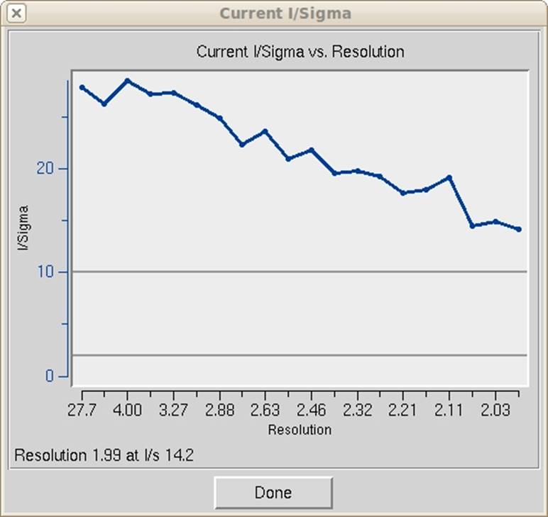
Figure 76. The I/Sigma vs. Resolution plot
The crystal dose button is to be used for X-ray sources with very high flux (typically synchrotron beamlines). It opens a new window Estimated Crystal Dose where you insert a correct Beam Flux value. The program runs a simulation estimating how radiation damage will cause the I/σ values to decrease at the end of data collection and shows the result as on the I/σ vs. resolution for Current and Last Frame plot (Figure 77). Note that this analysis requires the sequence of the protein in the crystal, which can be added by clicking the edit project button on the Project tab.
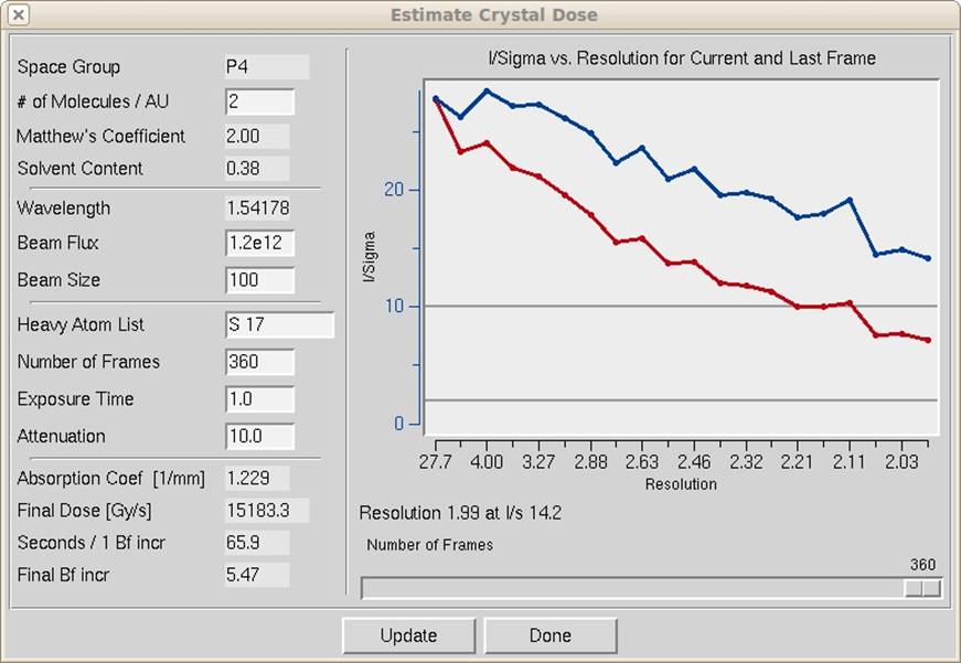
Figure 77. The Estimated Crystal Dose window
Simulation
The simulation utility predicts the number of overlaps for a data collection strategy as a function of frame width, distance, and oscillation range. This is particularly important if your crystal has high mosaicity or long unit cell axes. In those cases, the spots from some frames may have adequate separation, but then subsequent frames may be rendered useless by overlapping spots as (for example) a long axis that is perpendicular to the spindle axis rotates into a position parallel to the beam. The simulation utility allows you to simulate an entire data collection run, to view the potential overlaps, and then to adjust your data collection parameters before the crystal is exposed and time and valuable crystals are wasted. It is really quite useful.
Once the Omega Start and Omega End are input, click on the simulate run button. A mouse click on the Strategy plot will change these values to those that correspond to the cursor position in the plot. You will see two things. First, a plot will be drawn with red and blue lines (which may overlap), corresponding to the percentage of fully and partially recorded reflections that are predicted to be overlapped for each frame you plan on collecting (Figure 78). Remember, if a reflection is overlapped on another, it will not be useful for your data set and be excluded during integration and scaling. Second, on your Image Display image window, a new series of predicted reflections will be displayed, corresponding to each frame in your simulated data collection run. Obviously, since you haven't yet collected the data, the underlying diffraction image will not change or correspond to the predicted reflections, but that is OK (this is just a simulation). This will show you visually how your diffraction image will index over the data set collection.
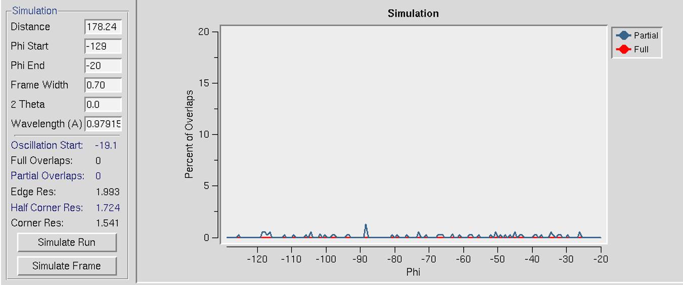
Figure 78. The Simulation window with almost no overlaps
The thing to pay attention to is the percentage of overlaps. Typically, you would like to lose no more than 5% of the reflections to overlap. This is where the simulation is useful. In the control box, you can replace the original frame width with a new value. Got a lot of overlaps? Decreasing the frame width can reduce problems with overlaps, so decrease this value and simulate the run again by clicking on the simulate run button. Examine the results; the overlaps should decrease. If you only have a few overlaps and want to increase the percentage of fully-recorded reflections, increase the frame width, and simulate the run again. Typically at some point, you will find a reasonable frame width (0.2-1.0° for macromolecules and 1.0-5.0° for small molecules) that yields an acceptably low number of overlapped reflections. This is not guaranteed, of course, since large unit cell axes and high mosaicity can conspire to ruin a run despite your best intentions.
Another way to decrease the number of overlaps is to increase the crystal-to-detector distance. As the detector is moved back, the spot separation should increase, and the percentage of overlaps will decrease. Naturally, this will limit how high the resolution of the data that can be collected, but it is worth trading off higher resolution data to ensure you can determine the structure. High-resolution data that can't be processed is useless. Perhaps you are one of the unlucky people that have the triple whammy of high resolution, large unit cell, and high mosaicity. In that case, you will be perpetually frustrated, but at least you will be able to develop the most rational data collection plan before exposing your crystals to an excessive amount of radiation. At some point, an acceptable compromise should be reached. You can also consider collecting multiple oscillations of data with varied data collection parameters and then scaling the sets together.
Once you have settled on an Omega Start, Delta Omega, Distance, and Frame Width, you can input these values into the control software for the data collection run and begin your data collection. Typically, the whole strategy and simulation exercise should take only a couple of minutes or less. It's actually easier to do it than to read about it!
If you are working with a precious crystal, it may be a good idea to collect a few frames using the strategy you have devised and check the strategy again. If anything is wrong, you can stop the data collection before you've irradiated the crystal too much. Errors or inaccuracies in the strategy or simulation, when they do occur, usually arise from an inaccurate estimation of the mosaicity or the unit cell axes, especially when these are derived from just a few frames.
Combining simulation runs to generate a cohesive strategy
The lower two plots, Completeness vs. Resolution, and Average and Cumulative Redundancy vs. Resolution (Figure 79), initially show statistics for a single simulation.
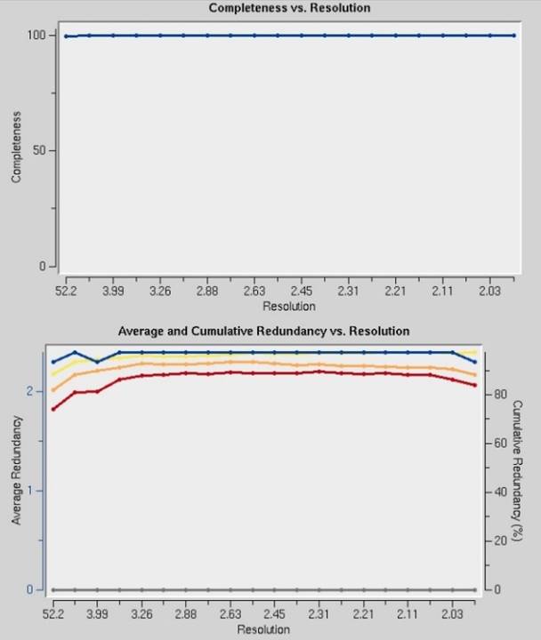
Figure 79. Completeness and Redundancy vs. Resolution plots
Sometimes due to hardware limitations, it is not possible to collect a complete data set while using a simple strategy, and you will have to combine several "wedges" of data to get a complete dataset. A short description of each simulation run will appear in the panel next to the combine button (Figure 80). The completeness in low (l) and high (h) resolution shells is shown above the combine button. You may select any combination of simulated runs by checking or unchecking the appropriate boxes next to each simulation run (each run will be selected by default). By clicking the combine button, you will obtain statistics and plots for a combination of the selected runs. You may remove all simulated runs from the last panel by clicking the clear button. If your version of HKL-2000 is configured with the data collection module, the setup dc button exports a chosen strategy to the Collect tab of the main HKL-2000 window.

Figure 80. The Combine panel