This tutorial shows you the automatic features of HKL-3000 that will allow you to go from raw diffraction data to a fairly complete molecular model with a very limited amount of intervention. This process works with a high percentage of data sets, so please give it a try. You can download a printable version of the text found beneath the video with images or a read-along version of the script that has thumbnails aligned with the script for the video.

Welcome to HKL Research’s “Introduction To Automatic Structure Solution Using HKL-3000”. This video focuses on using the automatic features built into HKL-3000 to go from raw diffraction data to an almost complete structural model using the single-wavelength anomalous diffraction (SAD) method. Data processing and scaling is identical in HKL-2000 and HKL-3000. For the purpose of this tutorial, we streamline this process using HKL’s automatic scaling procedure.  If you are interested in processing the data step-by-step, see the link below or visit the HKL Research webpage for a detailed video tutorial of processing and scaling.  

The data for today’s tutorial is available at proteindiffraction.org. A link is provided below. Search using the keyword ‘Workshop’ to find several excellent data sets. The one that we will work with today is 1WQ6, the nerve homology 2 domain of ETO. When you download the data from proteindiffraction.org, it will come with the site file that defines the detector setup. This file can either be placed in the HKLINT directory, or you can import it directly from the data directory.

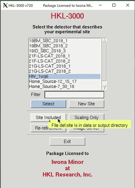
When you start HKL, you are first presented with a list of experimental sites.  The site definition contains information about the X-ray detector and other parameters that describe the experimental setup. The most important parameters are the type of detector, goniostat, and the position of the direct beam.  If your site definition is installed in HKL’s HKLINT directory, you can select the site from the screen that opens when you start HKL. The 1WQ6 data was collected using an ADSC-Q4 detector, so we could select this site. Instead, let me point out another HKL function. If a copy of the site file is in either the data directory or the output directory, you can select ‘Site Included”. This can be very convenient if you don’t have access to your network’s HKLINT directory.

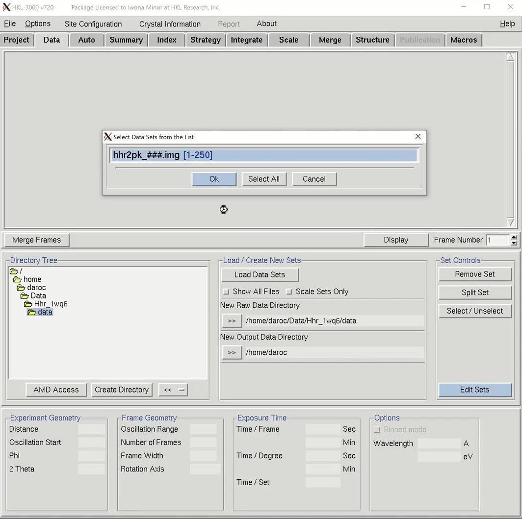
After the site selection screen, you are presented with the Data tab. This is where you specify the location of the data and select the sets of data to work with.  Use the Directory Tree on the left to navigate to and select the directory where the diffraction images are and click the double arrow button in the “New Raw Data Directory” field. Then click the load data sets button to see a list of the available data sets. This project has 250 frames of data available. When using the automatic scaling procedure, you do not need to select the output directory. You can verify that the site file was loaded correctly by displaying the first frame using the Display button. If the image doesn’t look like a diffraction image, your site file isn’t right.

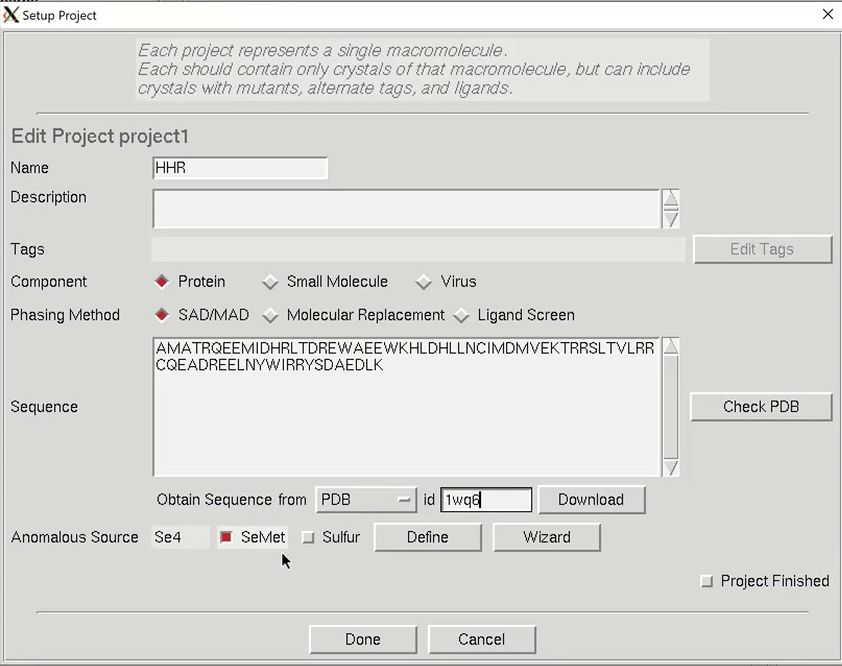
The structure solution module of HKL-3000 needs to know some basic information about your project in order to help you solve the structure. Change to the Project tab at the top of the main HKL window and click the Edit Project button to load the necessary information.

The minimal information that HKL needs is the type of macromolecule you are working with, the phasing method, the sequence, and the source of the anomalous signal. Although you can cut and paste the sequence, HKL can import it and some other information from various databases. Select the database using the drop-down menu labeled Obtain Sequence From and type the id associated with that database in the id field. Click download to fetch the sequence.

We will solve the structure using selenomethionine, so select the SeMet option, which will fill in the anomalous source field and the number of selenium atoms. Close the “Setup Project” dialog by clicking Done. The completed information now appears in the Project window.

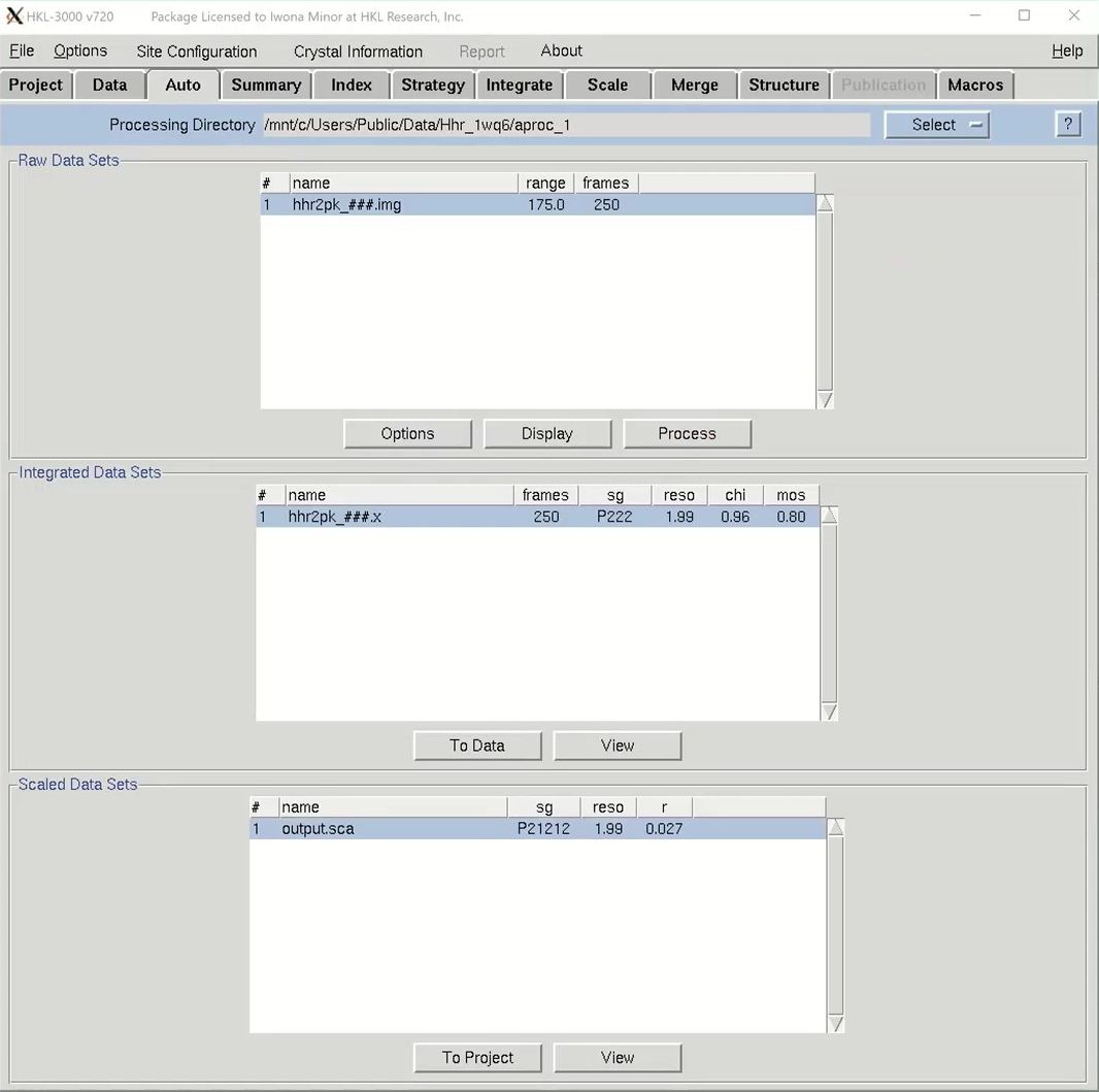
We are now ready to proceed to the automatic scaling procedure, so select the Auto tab. The dataset will be listed in the Raw Data Set frame. There are some options, but the defaults are usually sufficient. If you want to see the data, click the display button, but this is not necessary with the automatic processing. To get started, just click process. The stages will be displayed on the left side.  The program will peak search, index the data in different Bravais lattices and then integrate the data in the most likely lattice. Some integration statistics will appear in the Integrated Scaling Sets window as it is processed. When scaling is done, the spacegroup, resolution and Rmerge will be shown in the Scaled Data Sets window. If you have gone through the manual data processing and scaling tutorial, you might remember that this data always needs to be reindexed to get the screw axes on the right crystallographic axes.  The automatic processing will do this for you. To see the Scaling Graphs and Statistics you may be familiar with, click the View button at the bottom of the window. If you are satisfied, click To project to tell HKL you accept the results. These scaling results will now appear in the Project tab.

We are now ready to solve the structure using the Structure tab. Because we have defined the phasing method as SAD/MAD, the contents of the Structure tab will be specific for this method. On the right, we see some information about the project. Most of this is either set or based on information in the Project tab. HKL-3000 will automatically estimate the number of molecules in the asymmetric unit (ASU), the Matthews coefficient, and the solvent content.

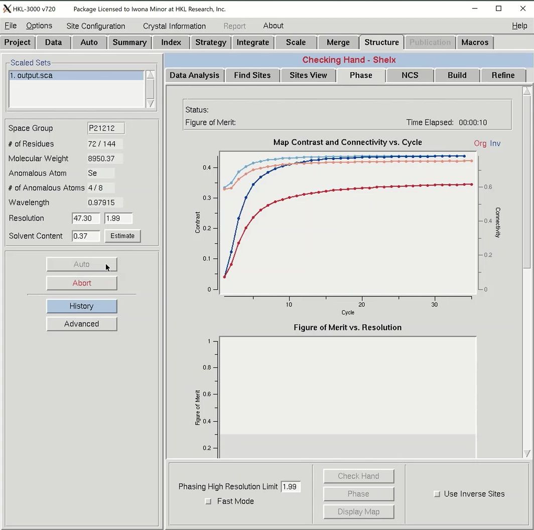
Click the Auto button to start the automatic building process. Analysis of the quality of the anomalous signal is done by the SHELXC and TRUNCATE programs. Determination of the heavy atom substructure is performed by SHELXD. Determining the hand of the substructure solution is done running SHELXE once with each hand of the data and comparing the map connectivity and contrast for each hand. Phasing, phase extension, and density modification are performed by SHELXE and MLPHARE.

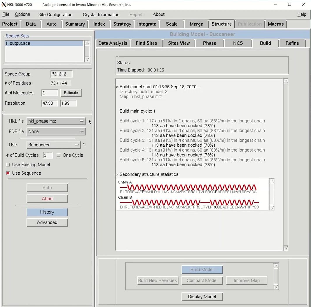
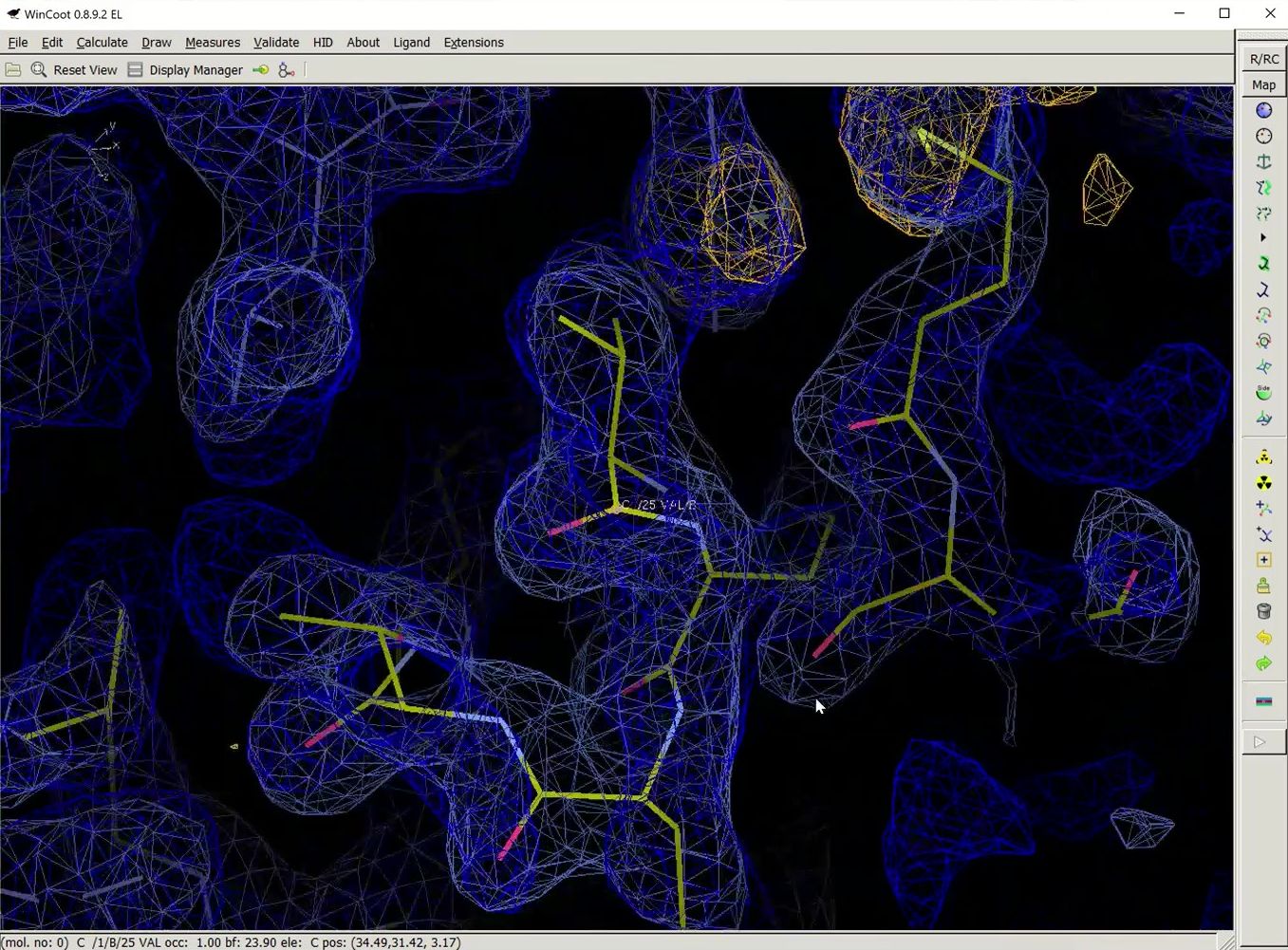
Once phasing is done, HKL will attempt to build a model using BUCCANEER. Once building has been started, COOT will launch to show you the quality of the initial phases. Maps and the substructure sites will be displayed. You may have to use the “Go To Atom” option to find the substructure. The experimental density map will be displayed in blue and the anomalous density map will be displayed in orange. The peaks of the anomalous density map should correlate with the sites.

The building process will have three building cycles, each followed by a round of refinement in REFMAC. For each cycle, the number of residues built and docked will be displayed, as well as the number of chains that contain them. After each main cycle, the secondary structure of the current model will be displayed along with the sequence. Each cycle of building will be followed by rounds of refinement in Refmac, and the R-values and the FOM from these cycles will be displayed.

Once building is complete, another session of COOT will open. This time, in addition to the substructure solution, anomalous difference map, and the density modified map, hopefully you will also see a fairly complete model and the refined 2Fo-Fc map.

We hope that you find the automatic features of HKL useful.  They won’t work in every case, but you should definitely give them a try. More in-depth tutorials for HKL are available on this channel and at the HKL Research web site.